The exact waveform needed can be generated by keying in
a mathematical equation [Y = f(t)] that precisely describes
the waveform amplitude, frequency, shape and duration.
With a few more keystrokes, noise, glitches, and other
forms of distortion can be added to simulate virtually any
real-world signal. Function keys such as SIN, Y
X
,
INTegral, LOG, and ARCTAN minimize the number of
keystrokes required. Mnemonics such as FOR, AT, and
TO simplify the description of complex, multi-segment
waveforms. Scientific notation and the metric prefixes M,
K, m, µ, and n not only ease numeric entry, they also allow
the equation to be written in the user’s language.
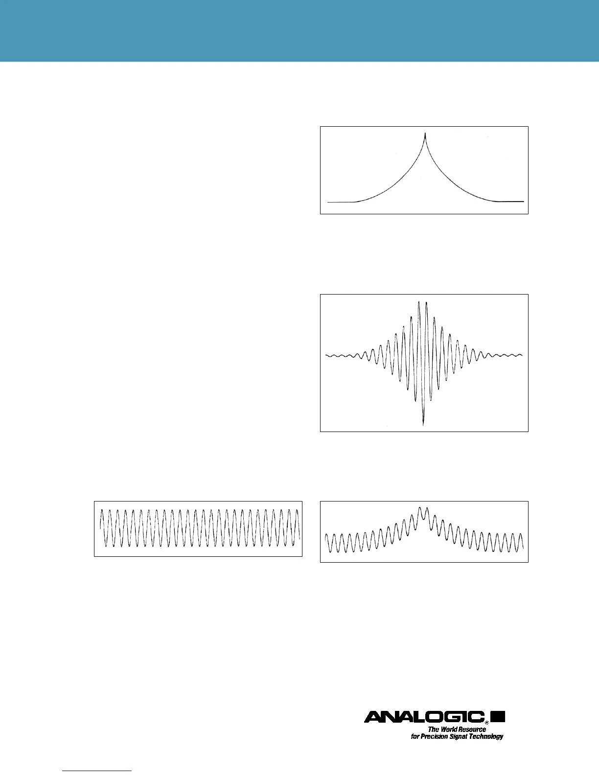
The waveforms illustrated in Figures 1 through 4 show
the creation of complex wave shapes by adding or multi-
plying ordinary math functions. These examples show the
relative ease of mathematically defining complex wave-
forms that precisely simulate natural phenomena. The
Analogic Model 2020 introduced Math Equation Entry to
the instrumentation marketplace, and has proven its versa-
tility and simplicity in a great variety of lab and manufac-
turing applications.
While Math Equation Entry enables the operator to pro-
duce nearly any desired waveform, several other methods
of definition are provided: computer download; data
download from the Model 6500 Waveform Analyzer,
standard functions with real-time menu control of ampli-
tude, symmetry, etc.; quantified noise added to a wave-
form; point and line segment entry; and scope draw for
waveform touchups.
Figure 1. Basic 10 kHz sine wave: F1 = SIN(10K*t)
Figure 2. Natural Transient envelope with peak at 1 ms: FOR
1m ARCSIN(a*t) FOR 1m ARCSIN(a*(1m–t)2). Where “m”
means millisecond and “a” determines envelope amplitude.
Figure 3. Product of sine wave and envelope of
Figures 1 and 2.
Figure 4. Sum of sine wave and envelope of Figures 1 and 2.
 Loading...