Casio fx9750GII - Data Logger Experiment: Cooling; Cooling Experiment: Procedure and Analysis

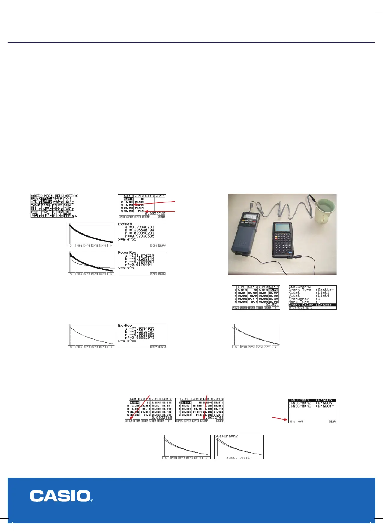
CONNECTION TO OTHER DEVICES
Procedure
Step 1: Heat approximately 250 ml of water. Bring it to the boil (approx 100° C).
Step 2: Place the thermometer probe into the cup of water after it has been heated.
Step 3: Set the rate of sampling of the EA-100 at 10 seconds and the number of samples to be taken at 200. Start the
data gathering with the EA-100 and relax for the next 33 minutes and 10 seconds.
Step 4: Transfer the data from the EA-100 to the calculator.
Step 5: Analyse the data collected as a time series. Fit an appropriate mathematical model to the data collected.
Step 6: Repeat the experiment with the spoon in the cup of water.
Analysis of the Results
The trend of the two curves displays the rate of cooling for the water. You may expect some results to differ as this is
dependent on different surface areas, different composition containers, addition of insulating materials, etc.
The analysis is done in the STAT icon, setting the statistical graph to be either a time series or scattergraph.
From the value of r
2
and comparing the two mathematical models,
the exponential model is the ‘best tting’.
Result #2: With the spoon: Transfer the data from the Data Logger
into List 3 and List 4 of the calculator.
Making comparisons between the cooling (i) without and (ii) with the spoon (radiator). The spoon ‘absorbs’ the heat –
heats up – (logarithmically). So the initial temperature is lower, but the cup of water cools at similar rates.
Without spoon: y = 81.985
-0.000355
With spoon: y = 77.958e
-0.000325
Result #1:
Without the
spoon:
An
exponential
model:
An
exponential
model:
The theoretical
model displayed.
y = 77.958e
-0.000325
A power
model:
Graphically, viewing both time series
or scattergraphs simultaneously:
Note: Newton’s Law of
Cooling states: That the
time a substance takes to
cool off depends on the
temperature difference
between the substance
and the surroundings.
Time (sec)
Temp (C)
select [F1]
[F6] will
draw the
two graphs.
then [F4]
Then turn StatGraph1
and StatGraph2 on
by pressing [F1].