®
Model No. AP-8209 Photoelectric Effect Apparatus
22
PART 2: Create labels for variables and units.
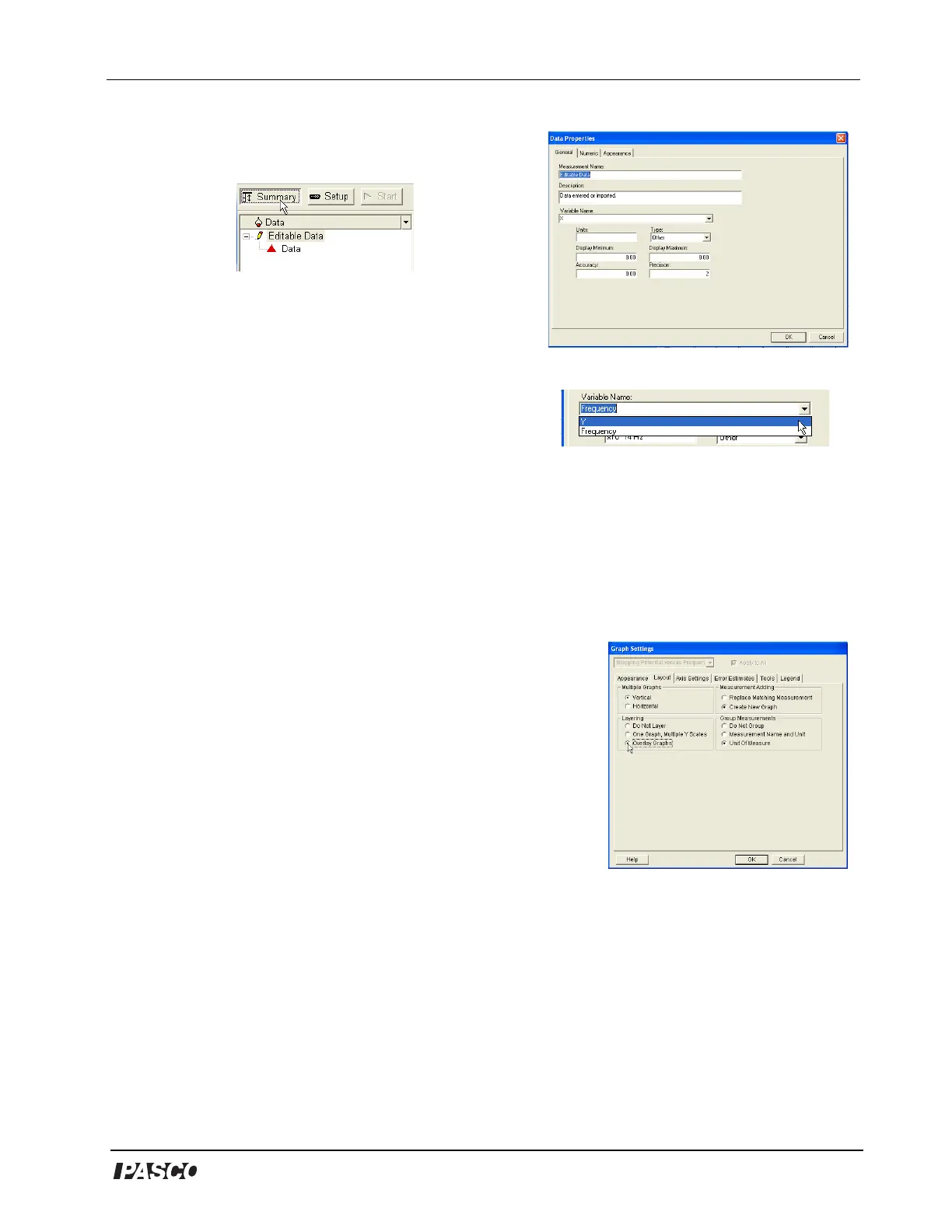
Double-click ‘Editable Data’ in the top of the Summary list to
open the Data Properties window.
Under ‘Measurement Name’ in the Data Properties window,
enter ‘Stopping Potential versus Frequency’ for Experiment 1.
Under ‘Variable Name’, highlight the ‘X’ and enter ‘Frequency’.
Under ‘Units’ enter ‘x10^14 Hz’.
Under ‘Variable Name’, use the menu button (down arrow) to
open the menu and select ‘Y’.
Enter ‘Stopping Potential’ as the ‘Variable Name’ and ‘V’ under
‘Units’.
Click ‘OK’ to close the Data Properties window.
PART 3: Enter X- and Y- data into the Table display.
Enter the first ordered pair (Frequency, Stopping Potential) in the
first row of the Table display using the following pattern:
<X- data> TAB <Y-data> RETURN.
Enter the rest of the ordered pairs of Frequency and Stopping Potential using the same pattern. Remember to press
RETURN after the last datum is entered.
As the ordered pairs are entered they will be plotted in the Graph display.
PART 4: Rename the Data.
In the Summary list, slowly double-click ‘Data’ (click-pause-click) to highlight ‘Data’. Enter an appropriate label
(e.g., 4 mm aperture) for the entered data.
PART 5: Analyze the Data.
In the Graph display, click the ‘Fit’ menu and select ‘Linear Fit’. In the
legend box that opens, the value of ‘m’ is the slope of the best fit line for
your data.
To plot more runs of data, select ‘New Empty Data Table’ from the
Experiment menu and repeat the procedure (PART 2 to PART 5).
In order to have the runs of data appear on the same plot in the Graph
display, double-click the Graph display to open the Graph Settings
window. Under the ‘Layout’ tab, click ‘Overlay Graphs’. Click OK to close
the window.
Data Properties
Select ‘Y’ in the ‘Variable Name’ menu
Overlay Graphs