Hardware and physical integration guideline A1 PCR sensors
Page 21 of 30
2024-02-07 © 2024 by Acconeer – All rights reserved
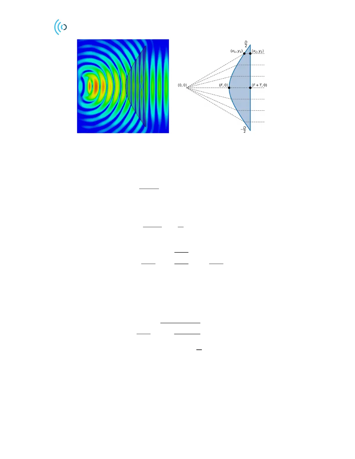
Figure 18. Hyperbolic lens with spherical E-field source (a) and corresponding ray model (b).
4.1.2 Convex-planar lens (Hyperboloidal lens)
By constraining the outer surface to planar we have 𝑥
=𝐹+ 𝑇, see Figure 18b. Equating the optical
path through a point (𝑥
,𝑦
) with the central path yields
(6)
Eq. (6) can be written as
(7)
where the coefficients are given by
𝑎=
𝐹
𝑛+ 1
,𝑏=
𝑛 − 1
𝑛 + 1
𝐹,𝑥
=
𝑛𝐹
𝑛+ 1
.
Observe that we have refraction only at the inner surface, that is, this is a single refracting lens. We
recognize Eq. (7) as a hyperbolic function shifted in the x direction by x
0
, hence the name hyperbolic
(2D) or hyperboloidal (3D) lens.
The central thickness of the lens can be shown to be
(8)
To generate a lens profile, we first choose a material 𝑛=
√
𝜖
. After this the diameter D and the focal
distance F is chosen to fulfill some maximum thickness requirement in Eq. (8). The lens profile is then
given by Eq. (7) by solving for 𝑦
=𝑦
(
𝑥
)
,𝑥
∈
[
𝐹,𝐹+ 𝑇
]
. A parametrization
𝑥
(
𝑡
)
,𝑦
(
𝑡
)
may be
required for generating the lens profile in CAD software. One such parametrization is
a
b
 Loading...