PT.RowAxisLayout xlTabularRow
PT.RowAxisLayout xlOutlineRow
PT.RowAxisLayout = xlCompactRow
In Excel 2007, you can add a blank line to the layout after each group of pivot items.
Although the Design ribbon offers a single setting to affect the entire pivot table, the setting
is actually applied to each individual pivot field individually. The macro recorder responds
by recording a dozen lines of code for a pivot table with 12 fields. You can intelligently add
a single line of code for the outer row field(s):
PT.PivotFields(“Region”).LayoutBlankLine = True
Applying a Data Visualization
Excel 2007 offers fantastic new data visualizations such as icon sets, color gradients, and in-
cell data bars. When you apply a visualization to a pivot table, you should exclude the total
rows from the visualization.
If you have 30 branches that average $50,000 in revenue each, the total for the 30 branches
is $1.5 million. If you include the total in the data visualization, the total gets the largest bar,
and all the branch records have tiny bars.
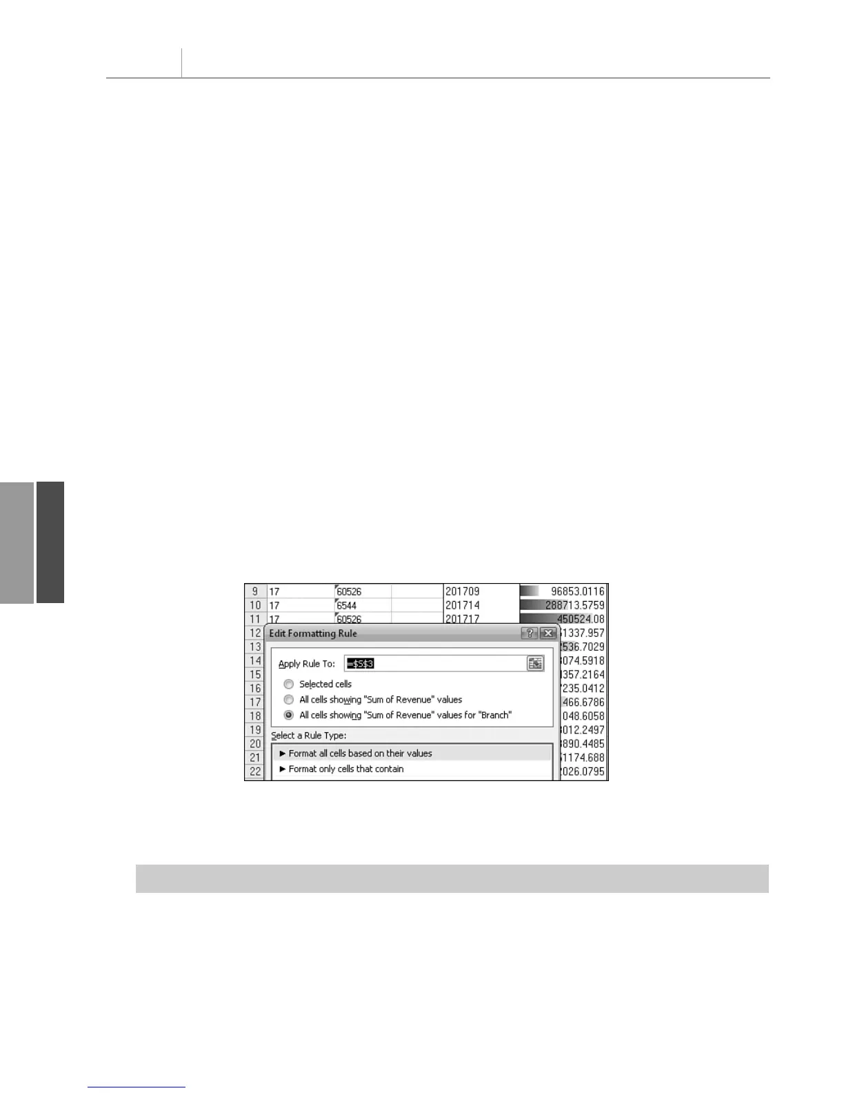
In the Excel user interface, you always want to use the Add Rule or Edit Rule choice to
choose the option All Cells Showing “Sum of Revenue” for “Branch,” as shown in
Figure 11.25.
Chapter 11 Using VBA to Create Pivot Tables
286
11
Figure 11.25
To create meaningful
visualizations in your
pivot table, exclude the
totals by choosing the
third option at the top of
this dialog box.
The code in Listing 11.11 adds a pivot table and applies a data bar to the revenue field.
Listing 11.11 Code That Creates a Pivot Table with Data Bars
Sub CreatePivotDataBar()
‘ Listing 11.11
Dim WSD As Worksheet
Dim PTCache As PivotCache
Dim PT As PivotTable
Dim PRange As Range
Dim FinalRow As Long
Set WSD = Worksheets(“PivotTable”)
12_0789736012_CH11.qxd 12/11/06 6:26 PM Page 286