Casio fx9750GII - Confidence Intervals (STAT) (Continued); Confidence Intervals: 1-P and 2-P Types

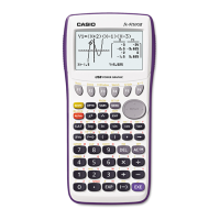
Condence Intervals 1-P type
Condence Intervals 2-P type
Is used in a similar way to the three types illustrated above when comparing two population proportions. Enter into the
statistics icon. Choose [INTR] [F4] then [F1] for Z-score. You now have a choice of 4 different options of condence
intervals. 1-S, 2-S, 1-P, and 2-P. This problem is a 2-P. So, press [F4].
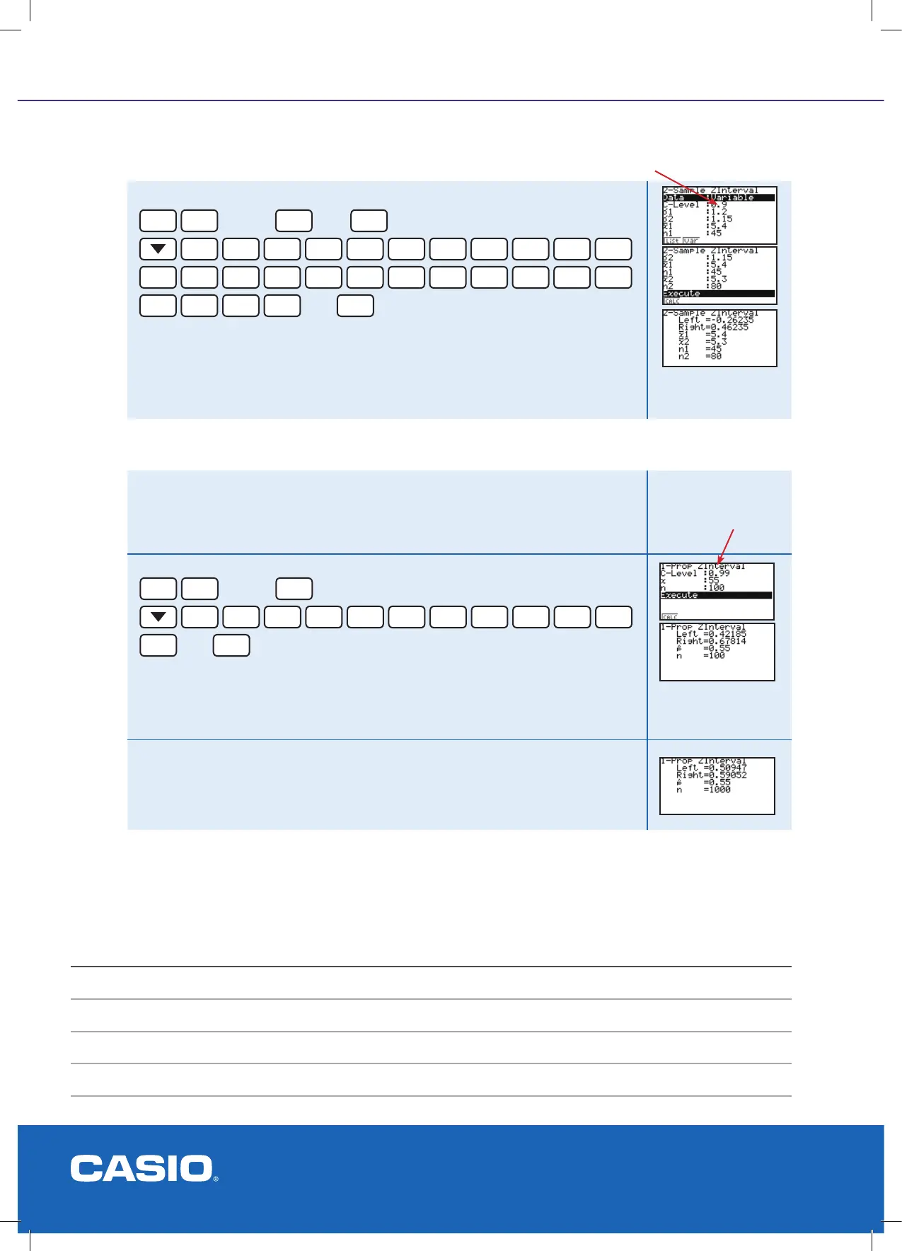
Condence Intervals 2-S type cont.
Example
Consider the following collected statistics. A sample was taken of worm
lengths at different areas of a market garden. Test at the 99% condence level,
to see what the ‘true’ population proportion is, if 55 out of 100 worms found
were greater than 9.3cm in length.
Result
F4 F1
Z-score
F3
[1-P]
0 . 9 9 EXE 5 5 EXE 1 0 0
EXE
then
EXE
This gives the interval [0.42185, 0.67814], hence the true population proportion
lies between 42% and 68% (2 sig.g.) of worms with a length greater than 9.3
cm.
[0.42185, 0.67814]
Remember: The larger the sample size the more accurate the sampling results.
i.e as n gets larger then the population statistic interval gets smaller.]
If n = 1000, then these results would be calculated - a much smaller interval
Example cont.
F4 F1
Z-score
F2
[2-S]
F2
[VAR]
0 . 9 EXE 1 . 2 EXE 1 . 1
5 EXE 5 . 4 EXE 4 5 EXE 5 . 3
EXE 8 0 EXE
then
EXE
This gives the interval [-0.26235, 0.46235], hence there is NO statistical
difference between the two samples as 0 is contained within the interval.
[-0.26235, 0.46235]
C-Level is at the
90% level
C-Level is at the
99% level
Notes:
NORMAL, BINOMIAL AND POISSON DISTRIBUTIONS