Casio fx9750GII - Confidence Intervals (STAT); Confidence Intervals: 1-S and 2-S Types

Condence Intervals [in STAT]
There are four types of condence interval calculations, one statistic (1-S), two statistic (2-S), one proportion (1-P), and
2 proportions (2-P).
Note:
You will have a choice of 4 different options of
condence intervals. 1-S, 2-S, 1-P, and 2-P. Use the
function to select the one that ts with the statistics.
Condence Intervals 1-S type
Condence Intervals 2-S type
Example
Consider the following collected statistics. A
sample was taken of worm lengths at different
areas of a market garden. Test at the 95%
condence level, to see if there is a statistical
difference between the worm lengths of this
sample and the ‘true’ population mean.
Sample
n = 56
Mean = 10.4
Standard deviation = 2.3
Result
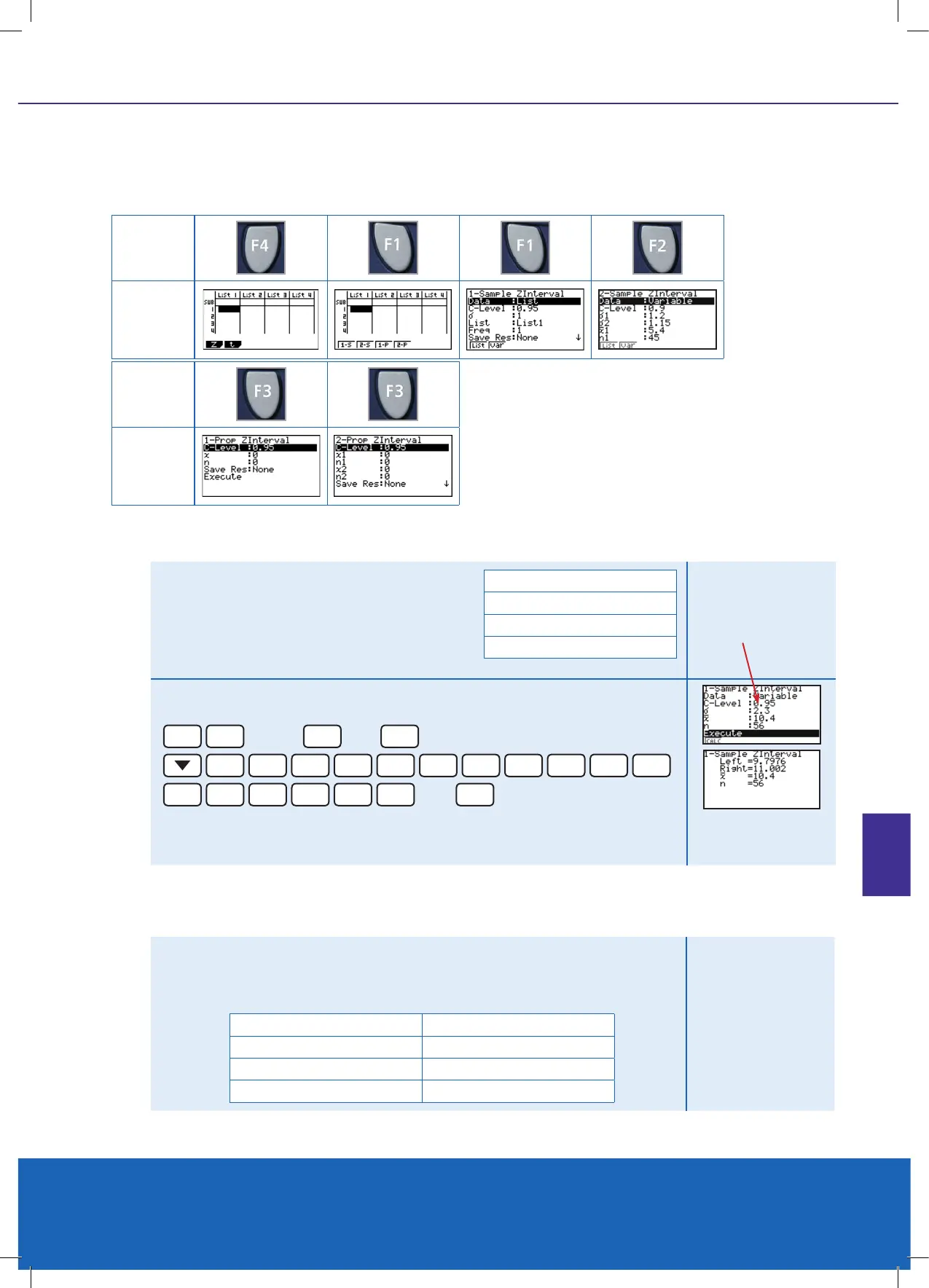
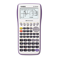
Set the calculator up so that inputted statistics is being used, not ‘raw data’. As
you can see raw data can be using in the LIST columns.
F4 F1
Z-score
F1
[1-S]
F2
[VAR]
0 . 9 5 EXE 2 . 3 EXE 1 0
. 4 EXE 5 6 EXE
then
EXE
This gives the interval [9.7976, 11.002], hence the ‘true’ population mean for the
worm lengths is in this interval, at the 95% condence level.
[9.7976, 11.002]
Example
Consider the following collected statistics. Two samples were taken of worm
lengths at different areas of a market garden. Test at the 90% condence
level, to see if there is a statistical difference between the worm lengths of two
samples.
Sample 1 Sample 2
n = 45 n = 80
Mean = 5.4 Mean = 5.3
Standard deviation = 1.2 Standard deviation = 1.15
Result
KEY
RESULT
KEY
RESULT
C-Level is at the
95% level
cont. on next page
fx9750GII
CHAPTER 8 | PG 71