Texas Instruments TI-82 - Page 11

11
G
RAPHING
T
ECHNOLOGY
G
UIDE
: TI-82
Copyright © Houghton Mifflin Company. All rights reserved.
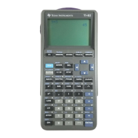
Figure 2.27: Trace on y = –x
3
+ 4x
Press TRACE to enable the left ◄ and right ► arrow keys to move the cursor along the function. The cursor is no
longer free-moving, but is now constrained to the function. The coordinates that are displayed belong to points on
the function’s graph, so the y-coordinate is the calculated value of the function at the corresponding x-coordinate.
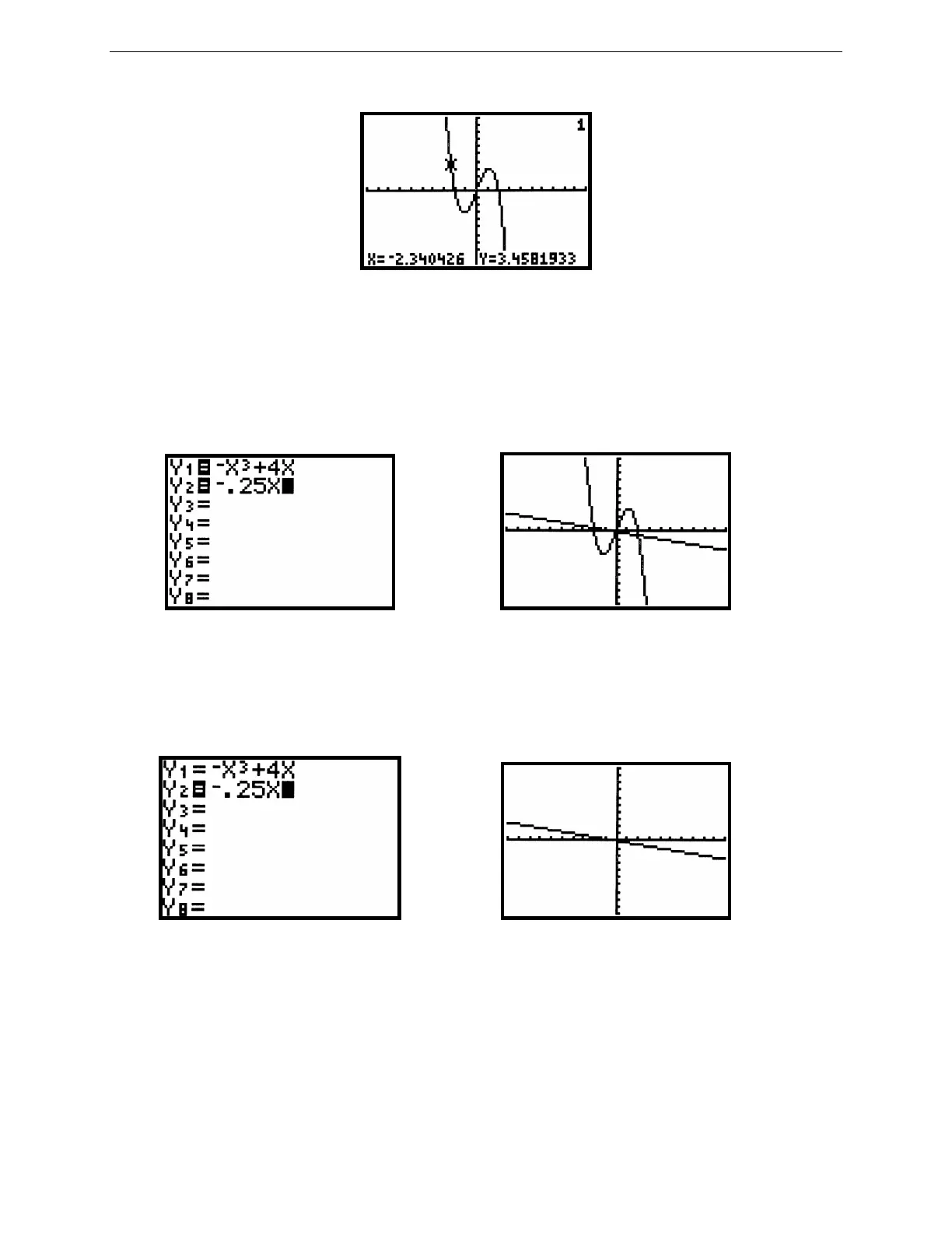
Now plot a second function, y = –.25x, along with y = –x
3
+ 4x. Press Y= and enter –.25x for Y
2
, then press
GRAPH.
Figure 2.28: Two functions Figure 2.29: y = –x
3
+ 4x and y = –.25x
Note in Figure 2.28 that the equal signs next to Y
1
and Y
2
are both highlighted. This means both functions will be
graphed. In the Y= screen, move the cursor directly on top of the equal sign next to Y
1
and press ENTER. This
equal sign should no longer be highlighted (see Figure 2.30). Now press GRAPH and see that only Y
2
is plotted
(Figure 2.31).
Figure 2.30: Y= screen with only Y
2
active Figure 2.31: Graph of y = –.25x
Many different functions may be stored in the Y= list and any combination of them may be graphed simultaneously.
You can make a function active or inactive for graphing by pressing ENTER on its equal sign to highlight (activate)
or remove the highlight (deactivate). Go back to the Y= screen and do what is needed in order to graph Y
1
but not
Y
2
.
Now activate Y
2
again so that both graphs are plotted. Press TRACE and the cursor appears first on the graph of y =
–x
3
+ 4x because it is higher up in the Y= list. You know that the cursor is on this function, Y
1
, because of the
numeral 1 that is displayed in the upper right corner of the window (see Figure 2.27). Press the up ▲ or down ▼