Texas Instruments TI-82 - Numerical Derivatives

32
G
RAPHING
T
ECHNOLOGY
G
UIDE
: TI-82
Copyright © Houghton Mifflin Company. All rights reserved.
To test the reasonableness of the conclusion that
21
lim
1
x
x
x
→∞
−
+
= 2, evaluate the function f (x) =
21
1
x
x
−
+
for several large
positive values of x (since you want the limit as x → ∞). For example, evaluate f (100), f(1000), and f (10,000).
Another way to test the reasonableness of this result is to examine the graph of f (x) =
21
1
x
x
−
+
in a viewing rectangle
that extends over large values of x. See, as in Figure 2.79 (where the viewing rectangle extends horizontally from 0
to 100), whether the graph is asymptotic to the horizontal line y = 2 (enter
21
1
x
x
−
+
for Y
1
and 2 for Y
2
).
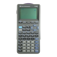
Figure 2.78: Checking
0
sin 4
lim
x
x
x
→
= 4 Figure 2.79: Checking
21
lim
1
x
x
x
→∞
−
+
= 2
1.11.2 Numerical Derivatives: The derivative of a function f at x can be defined as the limit of the slopes of secant
lines, so
0
()()
() lim
2
x
fx x fx x
fx
x
∆→
+∆ − −∆
′
=
∆
And for small values of ∆x, the expression
()()
2
fx x fx x
x
+∆ − −∆
∆
gives a
good approximation to the limit.
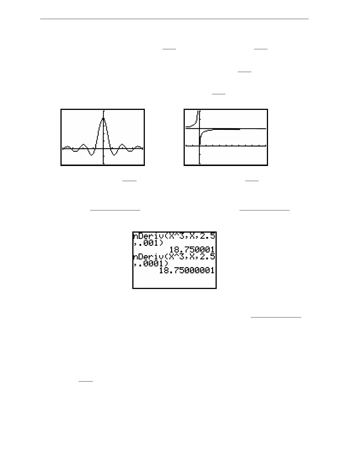
Figure 2.80: Using nDeriv(
The TI-82 has a function nDeriv( in the MATH menu to calculate the symmetric difference
()()
2
fx x fx x
x
+∆ − −∆
∆
.
So to find a numerical approximation to f´'(2.5) when f (x) = x
3
and with ∆x = 0.001, press MATH 8
X,T,θ
^
3,
ALPHA X, 2.5 , .001 ) ENTER as shown in Figure 2.80. The format of this command is nDeriv(expression,
variable, value, ∆x). The same derivative is also approximated in Figure 2.80 using ∆x = 0.0001. For most
purposes, ∆x = 0.001 gives a very good approximation to the derivative and is the TI-82’s default. So if you do use
∆x = 0.001, just enter nDeriv(expression, variable, value).
Technology Tip: It is sometimes helpful to plot both a function and its derivative together. In Figure 2.82, the
function f (x) =
2
52
1
x
x
−
+
and its numerical derivative (actually, an approximation to the derivative given by the