Texas Instruments TI-82

33
G
RAPHING
T
ECHNOLOGY
G
UIDE
: TI-82
Copyright © Houghton Mifflin Company. All rights reserved.
symmetric difference) are graphed. You can duplicate this graph by first entering
2
52
1
x
x
−
+
for Y
1
and then entering its
numerical derivative for Y
2
by pressing MATH 8 2nd Y-
VARS
1 1 ,
X,T,θ
,
X,T,θ
) as you see in Figure 2.81.
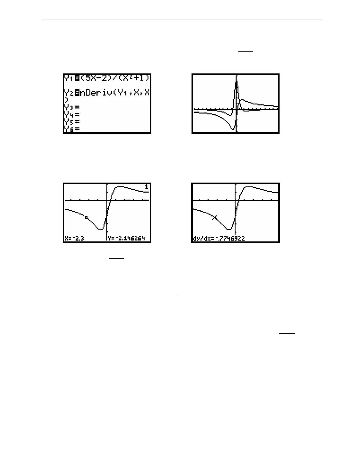
Figure 2.81: Entering f (x) and f´(x) Figure 2.82: Graphs of f (x) and f´(x)
Technology Tip: To approximate the second derivative f" (x) of a function y = f( x) or to plot the second derivative,
first enter the expression for Y
1
and its derivative for Y
2
as above. Then enter the second derivative for Y
3
by
pressing MATH 8 2nd Y-
VARS
1 2,
X,T,θ
,
X,T,θ
).
Figure 2.83 f (x) =
2
52
1
x
x
−
+
at x = –2.3 Figure 2.84: dy/dx
You may also approximate a derivative while you are examining the graph of a function. When you are in a graph
window, press 2nd CALC 6, then use the arrow keys to trace along the curve to a point where you want the
derivative (see figure 2.83 for the graph of f (x) =
2
52
1
x
x
−
+
at x = –2.3) and press ENTER. The TI-82 uses ∆x = 0.001
for this approximation.
1.11.3 Newton’s Method: With your TI-82, you may iterate using Newton’s method to find the zeros of a function.
Recall that Newton’s Method determines each successive approximation by the formula
1
()
()
n
nn
n
fx
xx
fx
+
=−
′
.
As an example of the technique, consider f (x) = 2x
3
+ x
2
– x + 1. Enter this function as Y
1
. A look at its graph
suggests that it has a zero near x = –1, so start the iteration by going to the home screen and storing –1 as x (see
figure 2.85). Then press these keystrokes:
X,T,θ
– 2nd Y-
VARS
1 1 ÷ MATH 8 2nd Y-
VARS
1 1 ,
X,T,θ
,
X,T,θ
)
STO►
X,T,θ
. Press ENTER repeatedly until two successive approximations differ by less than some predetermined
value, say 0.0001. Note that each time you press ENTER, the TI-82 will use its current value of x, and that value is
changing as you continue the iteration.