High PRF measurements
If a given pulse is narrower than the minimum analyzer
response time, it becomes impossible to measure a sin-
gle pulse. We must restrict ourselves to measurements
of a pulse train. In order to understand how such meas-
urements are possible, we must first have some funda-
mental understanding of how the analyzer treats an
incoming signal. This will allow us to anticipate the
instrument’s response to the presence of a discontinuous
signal such as a pulse.
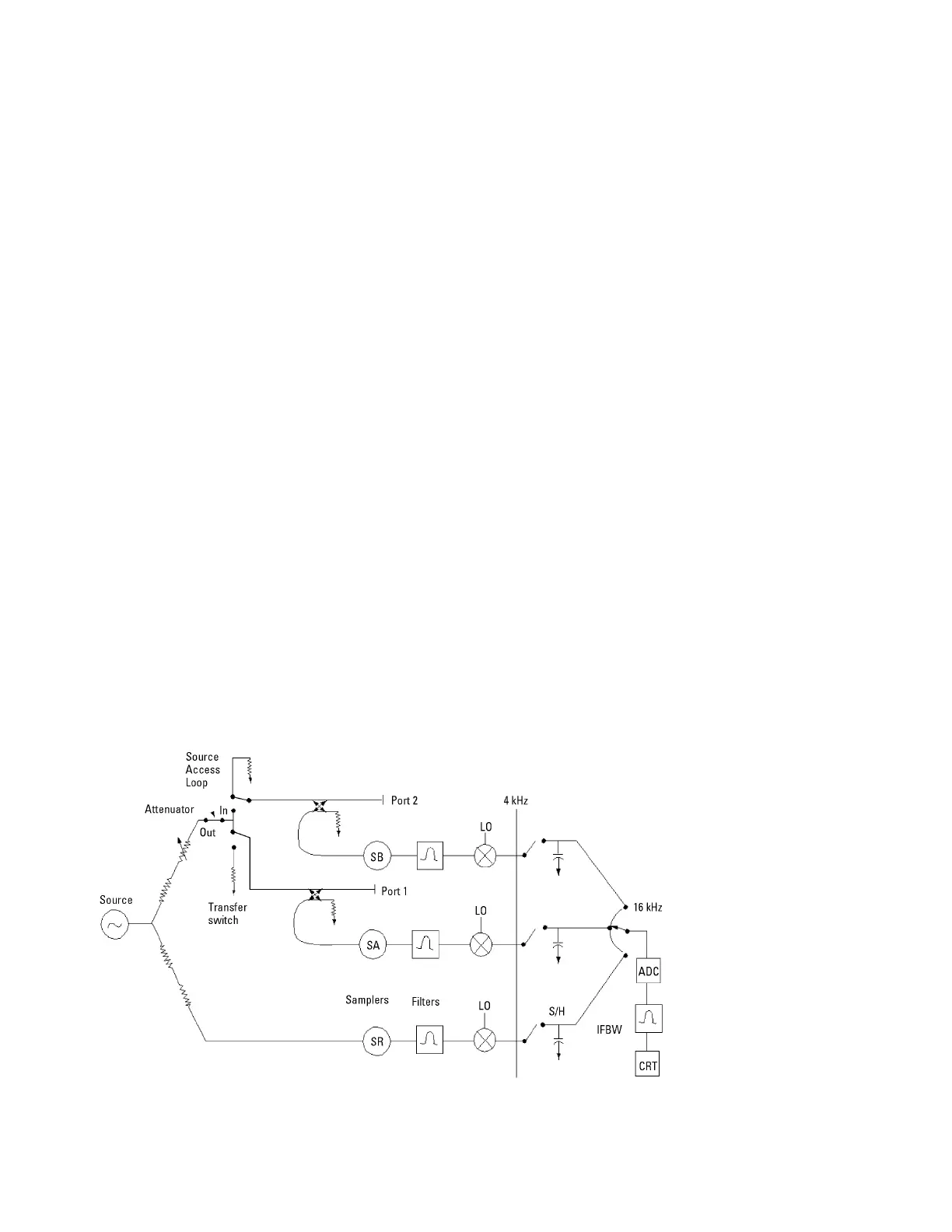
Looking at Figure 1, we see that in a normal measure-
ment, the source passes through the transfer switch,
through the port 1 coupler, and out to the DUT attached
to port 1. Transmitted signals pass through the DUT,
into port 2, through the port 2 coupler, and into sampler
B. Reflected signals return into port 1 and pass through
the port 1 coupler into sampler A. Signals that reach the
samplers are down-converted to an IF, filtered and
down-converted a second time to a 4 kHz IF. These sig-
nals are then digitized. After this step, all further signal
processing is done digitally.
Of all the elements in the signal path, it is the digital IF
bandwidth filter which exerts the greatest influence over
our pulsed signal. The IF bandwidth filter is a variable
bandwidth filter, ranging from 10 Hz to 6 kHz. As the
analyzer sweeps in frequency, the IF bandwidth filter
tracks along with the source, selecting only a narrow
segment out of the center of the IF signal bandwidth.
The relationship between the bandwidth of this filter
and the pulse repetition frequency (PRF) largely deter-
mines the response of the analyzer to a pulsed signal.
Figure 1. Network analyzer block diagram
Now consider the spectrum of a rectangular pulse train,
as shown in Figure 2. This is a MatLab
®
simulation of a
4 kHz continuous-wave (CW) signal, modulated by a rec-
tangular pulse train with a 200 Hz PRF and a 0.2 duty
cycle. Duty cycle for our purposes is defined as:
Duty Cycle ≡ Pulse Width / Pulse Period
This signal has already been downconverted to 4 kHz
and is ready to enter the IF bandwidth (IFBW) filter.
The left column of the figure shows the signal in the
time domain, while the right hand column shows the sig-
nal in the frequency domain. The first pair of diagrams
shows the pulsed signal without any IFBW filtering.
Notice that the presence of the modulating pulse trans-
fers energy out of the central "carrier" frequency and
spreads it into the sidebands. Multiple spectral lines are
present, and viewed in the time domain the pulse retains
a rectangular shape as it passes through the analyzer.
The analyzer responds to the pulse as you might expect;
part of the time an RF signal is on, and part of the time
the signal is off. Notice that the spectral lines are spaced
200 Hz apart, just equal to the PRF. Notice also that as
we move away from the center of the display, the first
minimum (or null) occurs at the fifth spectral line. Not
coincidentally, 1/5 equals our duty cycle (0.2). So, from
the spectral display we can deduce the characteristics of
the pulse train. These relationships hold true for any
rectangular pulse, regardless of frequency or duty cycle.
4
 Loading...