© -- --
© | y_1 | (y1 = f1(x1))
© | y_2 | (y2)
© c = M^(-1) * | y_3 | (y3) = f2(x3))
© | yp1 | (scaled value of f1'(x1))
© | yp3 | (scaled value of f2'(x3))
© -- --
©
© M^(-1) has been pre-computed. The following expression is all one line.
mat▶list([⁻.5,1,⁻.5,⁻.25,.25;.25,0,⁻.25,.25,.25;1,⁻2,1,.25,⁻.25;⁻.75,0,.75,⁻.25,⁻.25;0,1,
0,0,0]*[y_1;y_2;y_3;yp1;yp3])
EndFunc
The following example uses splice4() to splice two approximating functions.
Example: approximate the sin() function
Suppose we want to estimate sin(x) for 0 < x < 0.78 radians. We have found these estimating
functions:
for x > 0 and x < ~0.546 [18]
f
1
(
x
)
= k
1
$
x
3
+ k
2
$
x
2
+ k
3
$
x + k
4
k
1
=−0.15972286692682 k
3
= 1.0003712707863
k
2
=−0.00312600795332 k
4
=−4.74007298E − 6
for x > ~0.546 and x < 0.78 [19]
f
2
(
x
)
= k
5
$ x
2
+ k
6
$ x + k
7
k
5
=−0.3073521499375 k
7
=−0.04107647476031
k
6
= 1.1940610623813
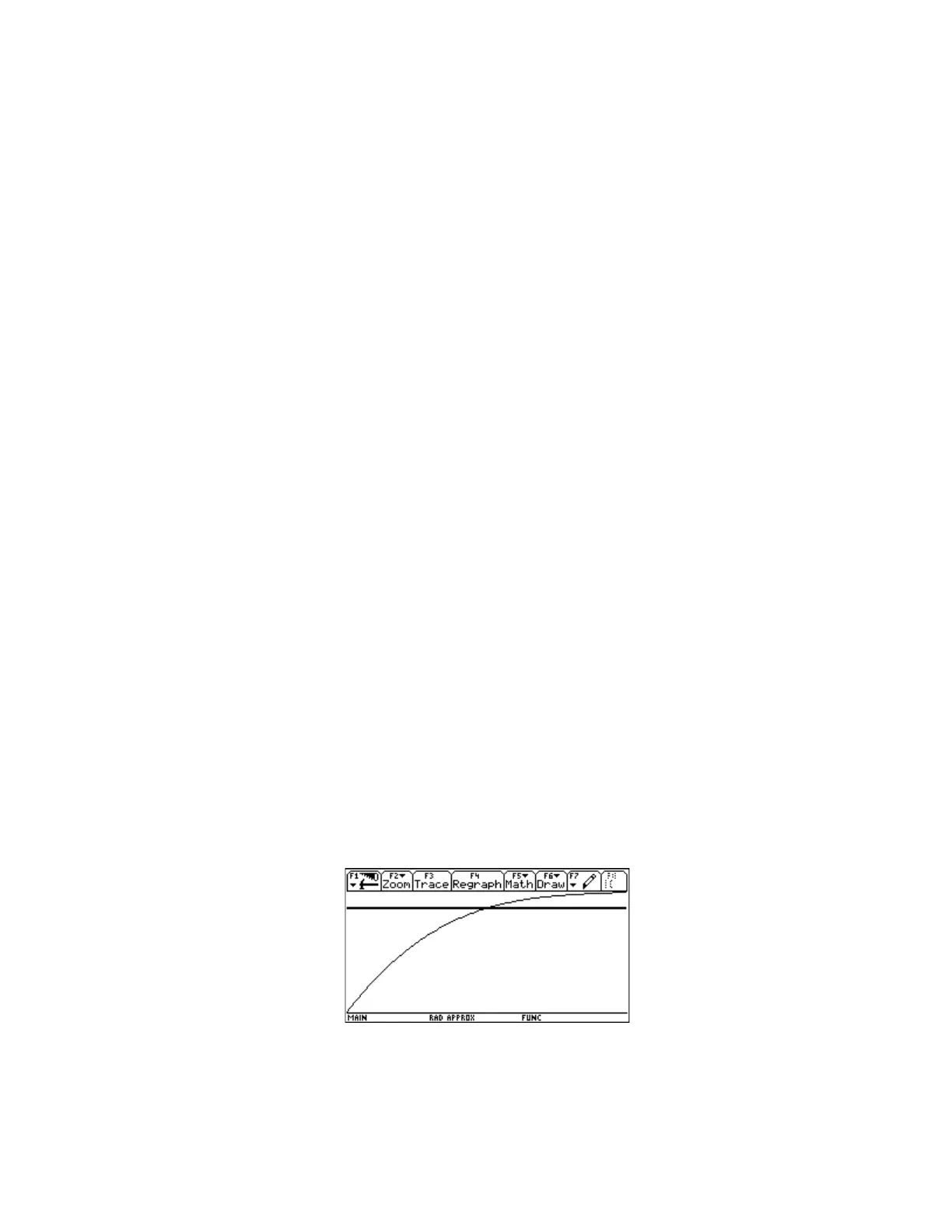
The first step is to set the center of the splice, x
2
. We want to set the splice center near the boundary
between f
1
(x) and f
2
(x), so as a starting point we plot the difference between the two estimating
functions, which is f
2
(x) - f
1
(x). We plot the difference instead of the functions themselves, because both
functions are so close to sin(x) that we would not be able to visually distinguish any difference. The plot
below shows the difference over the range 0.45 < x < 0.65.
6 - 98