a
4
= 0a5=−
4
375
a
6
= 0
a
7
=−
6364
1010625
a
8
= 0a
9
=−
275708
65690625
a
10
= 0a
11
=−
20793692
6897515625
a
12
= 0a
13
=−
−1335915116
596288828125
a
14
= 0
a
15
=−
7665058771652
4288702777734375
a
16
= 0a
17
=−
92763867329564
64330541666015625
and approximate values for the non-zero terms are
a
0
= 1 a
9
= -4.1970 6769 4210 6 E-3
a
1
= -0.6 a
11
= -3.0146 6399 3602 8 E-3
a
3
= -2.2857 1428 5714 3 E-2 a
13
= -2.2785 9555 2080 3 E-3
a
5
= -1.0666 6666 6666 7 E-2 a
15
= -1.7872 6742 5349 8 E-3
a
7
= -6.2970 9338 2807 7 E-3 a
17
= -1.4419 8797 2232 0 E-3
Note that asympexp() returns the coefficients as a list in the form {a
n
, a
n-1
, ..., a
0
}, so the expansion can
be evaluated as
polyEval(a,1/x)
where a is the list of coefficients. In general, you would keep finding additional terms until they started
to increase in value, then the best approximation would use all the still-decreasing terms. Even though
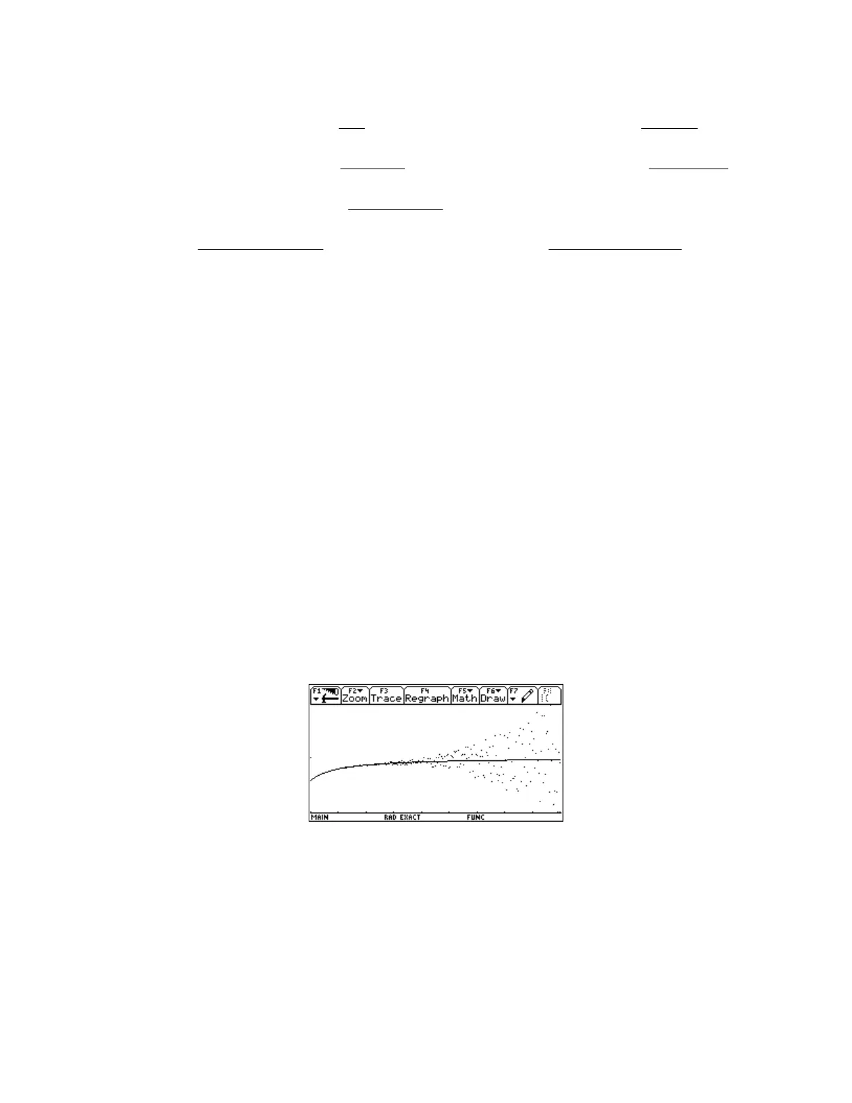
the terms above are still decreasing, I decided to check the expansion with the terms through a
9
. This
plot shows the original function as points, the asymptotic expansion as a solid line, on the interval x =
[100, 1000].
This is obviously a considerable improvement over the original function.
If we want to find both large and small values of the original function, we need to know the value of x at
which to switch to the asymptotic function. One starting point is to plot the difference of the two
functions, and switch to the asymptotic function before the round-off noise the original function begins.
I could just plot the difference of the two functions, but the dynamic range is so large that the round-off
noise would not be seen, so I plot the natural logarithm of the absolute value of the difference between
the two functions, which essentially gives me a plot with a logarithmic y-axis. It looks like this:
6 - 129