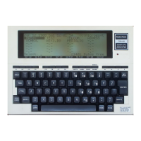
RUN the new program to confrrm that the trend line equation and the ftrst quarter
average ratio
to
trend are printed
as:
FORECAST
FOR
PERIOD X
IS
148.22463768116
+
8.4086956521739
*
X
QUARTER
1 RATIO
IS
.9230187061999
Ok
III
To predict sales into the future for quarter 1 of year 7, ftrst compute the trend line
forecast for period
25
(you can reduce the above ftgures to 3 or 4 decimal places):
PR
I
NT
148.225
+
8.4087
*
25
(ENTER)
the result will be 358.4425
Then multiply by the first quarter average ratio
to
trend
to
take seasonal fluctuation
into account:
PRINT
0.92
*
358.443
the answer will be 329.76756
Thus, 329.76756 would represent a prediction of quarter I sales in year 7, taking into
account both long term trend and typical ftrst quarter seasonal variation.
This experiment required the program to use every fourth number in the sales array
Y(X). This was easily accomplished with a slight change
to
the FOR statement
in
line
140:
140 FOR X = 1 TO N STEP 4
This change in the FOR statement tells the computer to increment the index variable X
in steps
of
4 starting with the value 1 until X reaches the upper limit
N.
Thus, X will
assume the values
1,
5,
9, 13,
17
and 21, which corresponds
to
the first quarter period
number in years 1, 2, 3, 4, 5 and 6 respectively.
Line
159 computes the ratio to trend for period X and then adds this to the sum of the
previous periods ratios.
Line
169 tests the value of the FOR statement index variable X to see
if
it has reached
the upper limit
N.
If it has not, the loop consisting of lines 140 to 160
is
repeated.
If
the index variable X has reached its upper limit, execution continues with line 170.
Line
179 prints the average ratio to trend for quarter
1.
Note that the numerical
expression R/6 within the PRINT list computes the average ratio by dividing the sum
of the ratios R by the number of ratios 6.
This experiment took into consideration the seasonality of quarter
1.
The next
experiment extends this concept
to
each of the four quarters.
96
 Loading...