41
www.agilent.com/find/esg
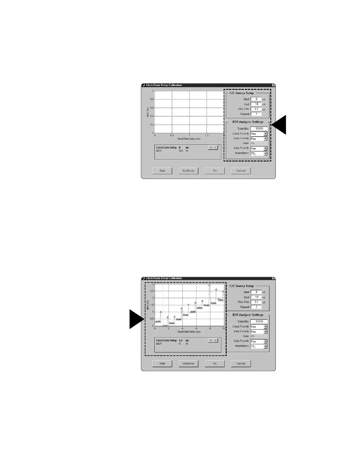
5. Configure the automated clock/gate delay calibration utility, Figure 45. In this example,
the clock/gate sweep end field is set to 10 us. Default values are used for the remaining
configuration fields.
Figure 45. Clock/Gate Delay calibration utility setup.
6. Once configured, select the Start button to generate the plot of BER vs. clock/gate
delay. The plot points are incrementally filled in as each test iteration is completed.
7. After the plot has been generated, a marker is automatically placed at the clock/gate
delay setting that yields the minimum BER, Figure 46. Notice that the plot looks similar
to a step function. With no impairments added to the signal, there is a range of approxi-
mately 1/2 a symbol period that yields the same BER results. In this case, the marker is
placed at the first BER minimum. When impairments are added to the signal, the plot no
longer looks like a step function. Instead, it looks like a series of parabolas, from which a
true minimum can be found. By initially performing the calibration without impairments
added to the signal, the clock/gate delay range for optimum BER can easily be determined.
As a result, when later performing clock/gate delay calibration on an impaired signal,
the sweep range can be adjusted accordingly.
Figure 46. BER vs. Clock/Gate Delay calibration results.
Basic Measurements
 Loading...