149
Either use the VIEWS Auto Scale option, or
change to the PLOT SETUP view and adjust it
so that it will display the data. This is not really
needed, since the line of best fit is what we
need and it will be calculated even if the data
doesn’t show.
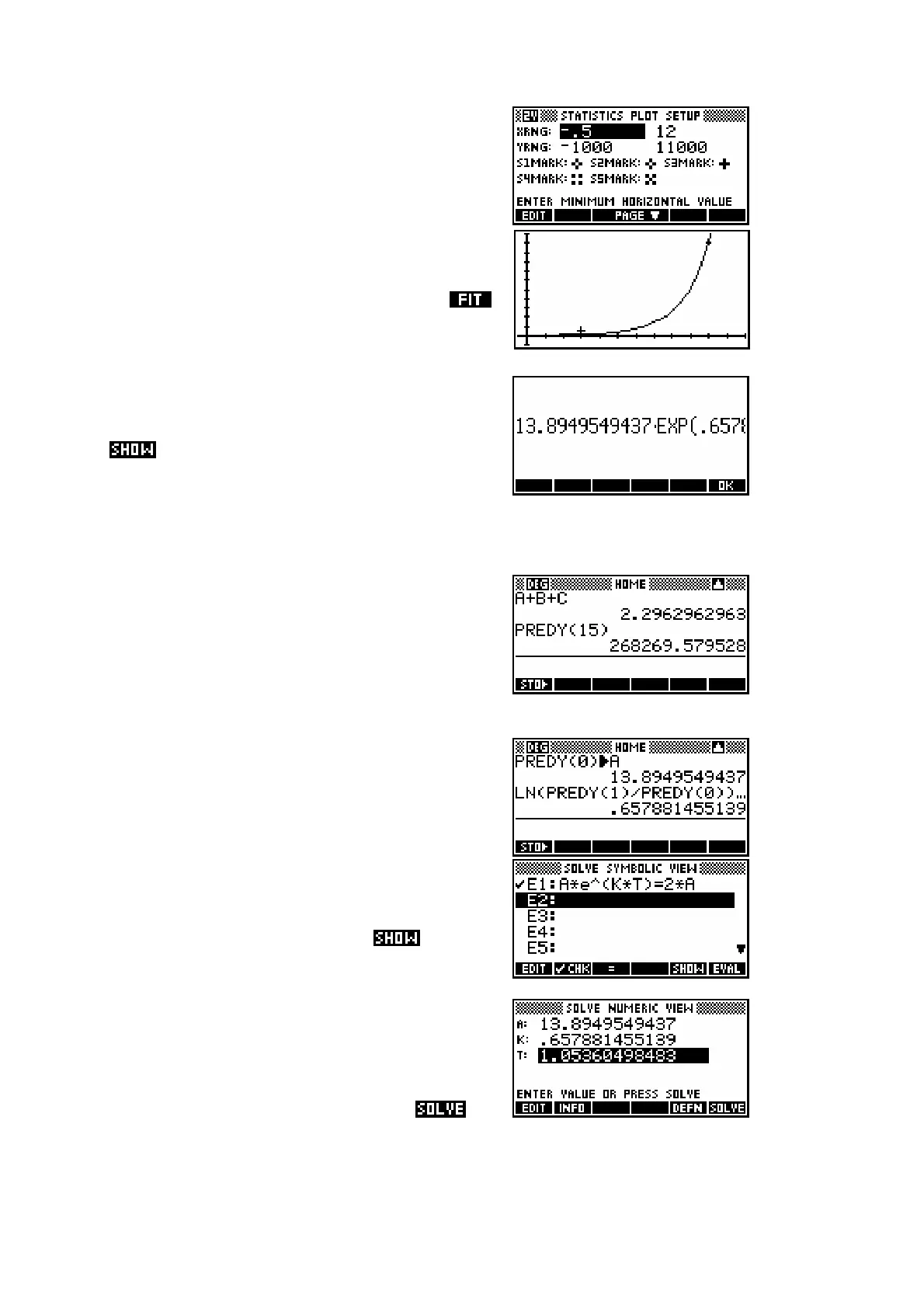
Now change to the PLOT view and press .
Wait while the line draws.
Change to the SYMB view, move the highlight
to the equation of the regression line and press
. Rounded to 4 dec. places, this gives an
equation of
0 6579
13 8950
t
Ne
⋅
=⋅ .
(ii) Predict N for t = 15 hours.
Change to the HOME view and use the PREDY
function or use the facilities in the PLOT view.
Result: 268 269 colonies.
(iii) Find t so that
0
2NN= .
The value of
0
N is the y intercept of the line of
best fit. These values from the curve of best fit
are not directly accessible but can be retrieved
using the PREDY function (see page 145). This
is shown in the screen shown right. Store the
results into memories A and K. This saves
having to re-type them from the screen.
Now switch to the Solve aplet and enter the
equation to be solved. Changing into the NUM
view, you should find the values of A and K
already defined (that was why we stored the
curve values into the appropriate memories),
so move the highlight to T and press .
Result: Doubling time is 1.0536 hours.
 Loading...