Quanser 3 DOF - Background; Modeling; Equations of Motion; Linear State-Space Model

2 BACKGROUND
2.1 Modeling
2.1.1 Model Convention
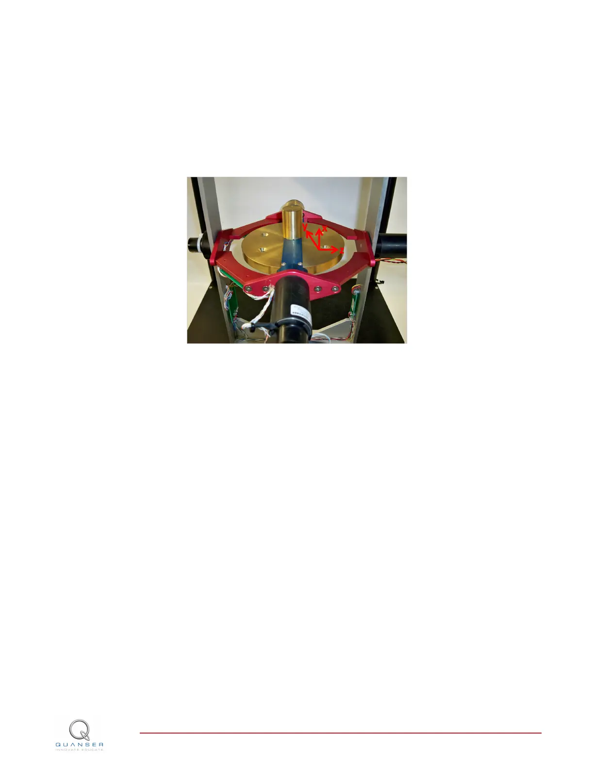
The reference coordinate frame for the 3 DOF Gyroscope is shown in Figure 2.1.
Figure 2.1: 3 DOF Gyroscope coordinate frame
2.1.2 Equations of Motion
The equations of motion representing the angular rate of the red gimbal, ψ, and the outer blue gimbal, θ, are ([1]):
J
y
¨
θ + h
˙
ψ = τ
y
J
z
¨
ψ − h
˙
θ = 0 (2.1)
where
J
y
= 0.0039 kg-m
2
J
z
= 0.0223 kg-m
2
h = 0.44 kg-m
2
/s.
The moment of inertia about the y-axis angle, θ, is J
y
and the moment of inertia about the z-axis angle (red gimbal),
ψ, is denoted as J
z
. The constant h is calculated based on the moment of inertia of the gyroscope rotor about its
own axis and its velocity. Because the outer gray rectangular frame is fixed, the only actuated axis is the y-axis. The
control input in the single-input single-output (SISO) system is the torque applied in the y-axis, τ
y
.
2.1.3 Linear State-Space Model
The linear state-space equations are
˙x = Ax + Bu (2.2)
and
y = Cx + Du (2.3)
where x is the state, u is the control input, A, B, C, and D are state-space matrices.
3D GYRO Laboratory Guide
v 1.1