Remark: When tuning the LQR, Q(2, 2) effects the red gimbal proportional gain while Q(1, 1) effects the red
gimbal derivative gain (which reduces the overshoot). Q(4, 4) affects the red gimbal integral gain which is used
to minimize the steady state error.
4. The Frequency control in the VI is already setup to generate a 0.1 Hz square wave reference.
5. Start the simulation by clicking on the white arrow button found on the top right hand corner of the VI (CTRL +
R).
6. Set the Amplitude control to 20 degrees to generate a step with an amplitude of 20 degrees (i.e., square wave
goes between ±20 which results in a step amplitude of 20).
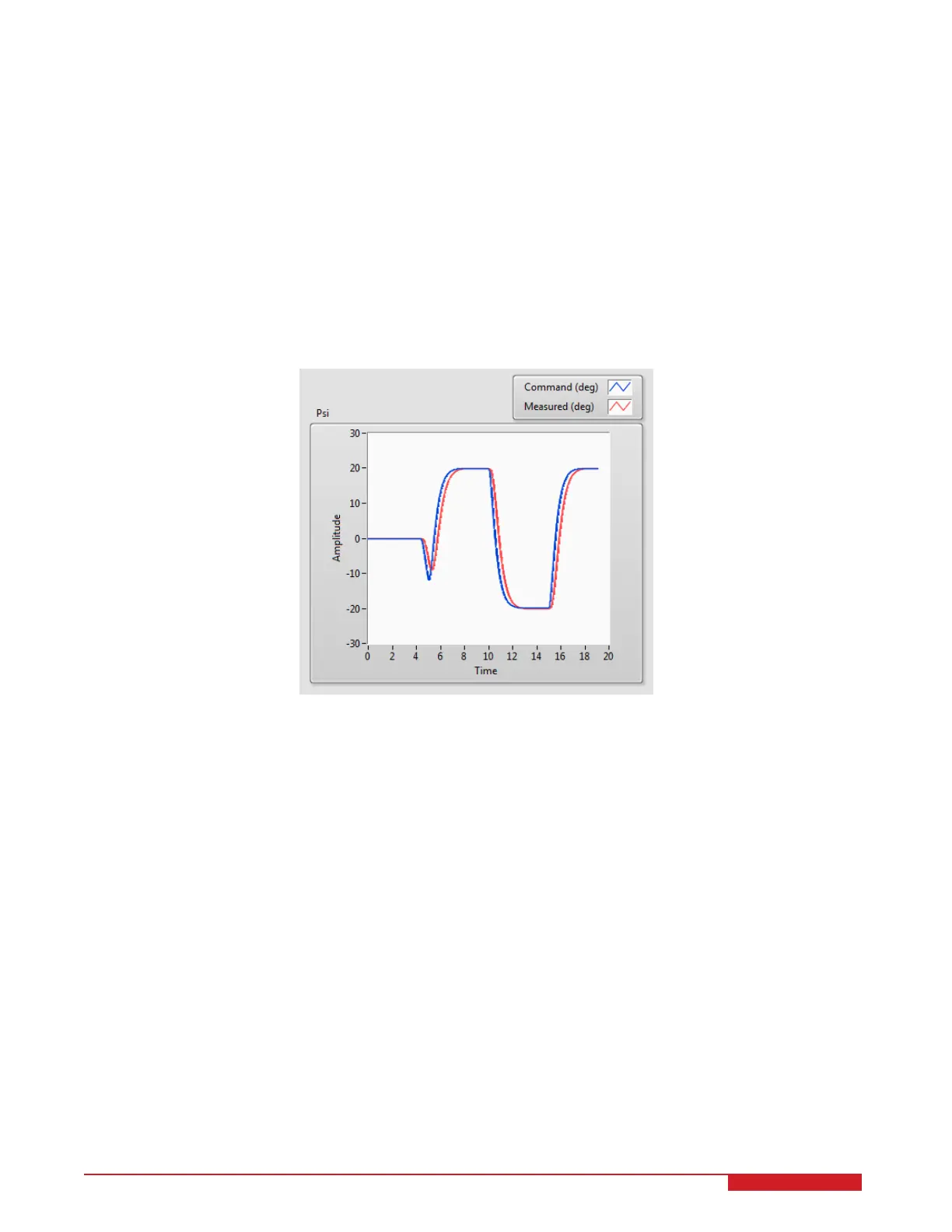
7. Go to the Psi Scope to view the red gimbal position command and actual values.
8. The scope should be displaying a response similar to Figure 3.2. Note that in the Psi scope, the blue trace is
the setpoint position and the red trace is the simulated position.
Figure 3.2: Simulated closed-loop response.
9. This is an iterative design process. You can go back and change your Q and R matrices, acquire a new control
gain K, on the fly while the simulation is running and see the resulting performance.
10. Click on the STOP button to stop running the VI.
3.2 Implementation
The 3D_GYRO_LQR VI shown in Figure 3.3 is used to perform the red gimbal position control on the 3D GYRO.
The VI contains drivers that interface with the DC motor and sensors of the 3D GYRO system.
IMPORTANT: Before you can conduct these experiments, you need to make sure that the lab files are configured
according to your setup. If they have not been configured already, then you need to go to Section 4 to configure the
lab files first.
3.2.1 Procedure
Follow this procedure:
3D GYRO Laboratory Guide 10