• Marginally stable systems have one pole on the imaginary axis and the other poles in the left-hand plane.
The poles are the roots of the system's characteristic equation. From the state-space, the characteristic equation of
the system can be found using
det (sI − A) = 0 (2.5)
where det() is the determinant function, s is the Laplace operator, and I the identity matrix. These are the eigenvalues
of the state-space matrix A.
2.2.2 Controllability
If the control input, u, of a system can take each state variable, x
i
where i = 1 . . . n, from an initial state to a final
state then the system is controllable, otherwise it is uncontrollable ([3]).
Rank Test The system is controllable if the rank of its controllability matrix
T =
B AB A
2
B . . . A
n
B
(2.6)
equals the number of states in the system,
rank(T ) = n. (2.7)
2.2.3 Linear Quadratic Regular (LQR)
If (A,B) are controllable, then the Linear Quadratic Regulator optimization method can be used to find a feedback
control gain. Given the plant model in Equation 2.2, find a control input u that minimizes the cost function
J =
∞
0
x(t)
′
Qx(t) + u(t)
′
Ru(t) dt, (2.8)
where Q and R are the weighting matrices. The weighting matrices affect how LQR minimizes the function and are,
essentially, tuning variables.
Given the control law u = −Kx, the state-space in Equation 2.2 becomes
˙x = Ax + B(−Kx)
= (A − BK)x
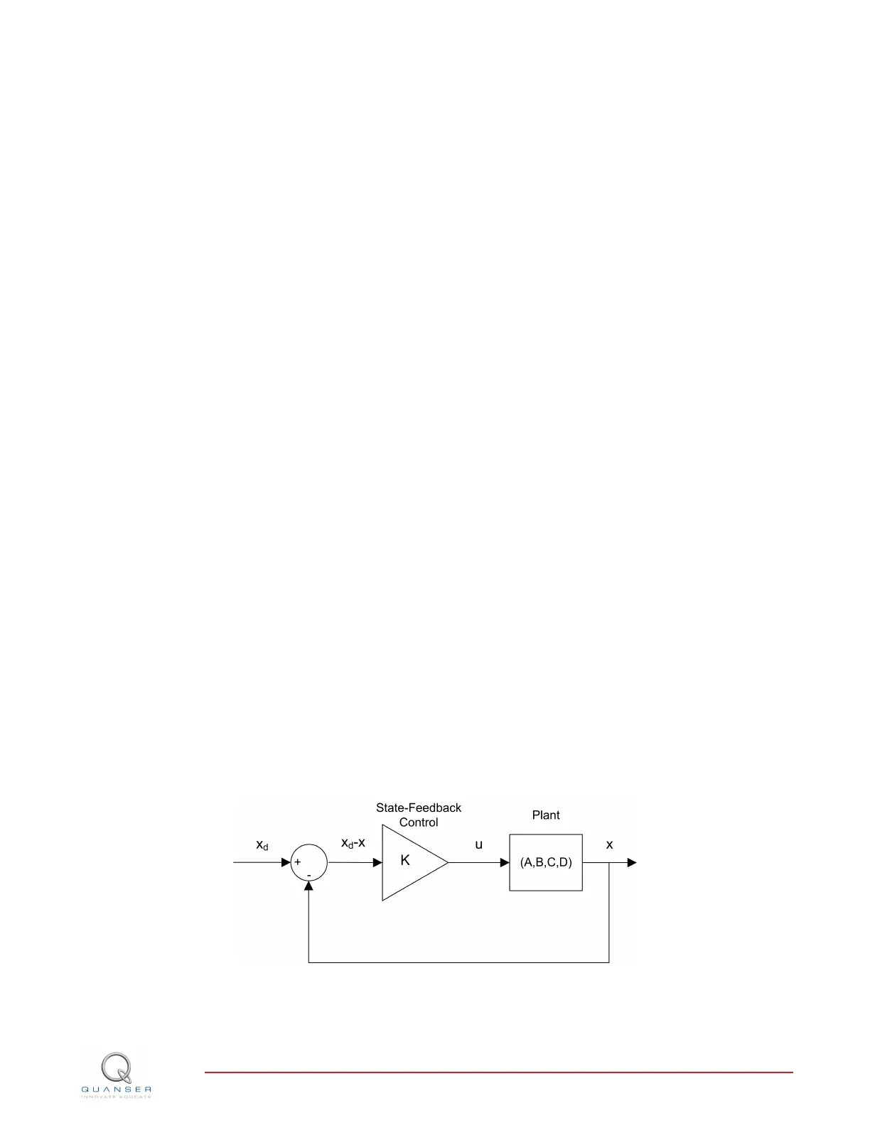
2.2.4 Feedback Control
The feedback control loop in Figure 2.2 is designed to stabilize the red gimbal to a desired position, ψ
d
.
Figure 2.2: State-feedback control loop
The reference state is defined
x
d
=
0 ψ
d
0 0
3D GYRO Laboratory Guide
v 1.1