CHAPTER 2. ALPY 600 - SPECTROSCOPY IN SLIT MODE
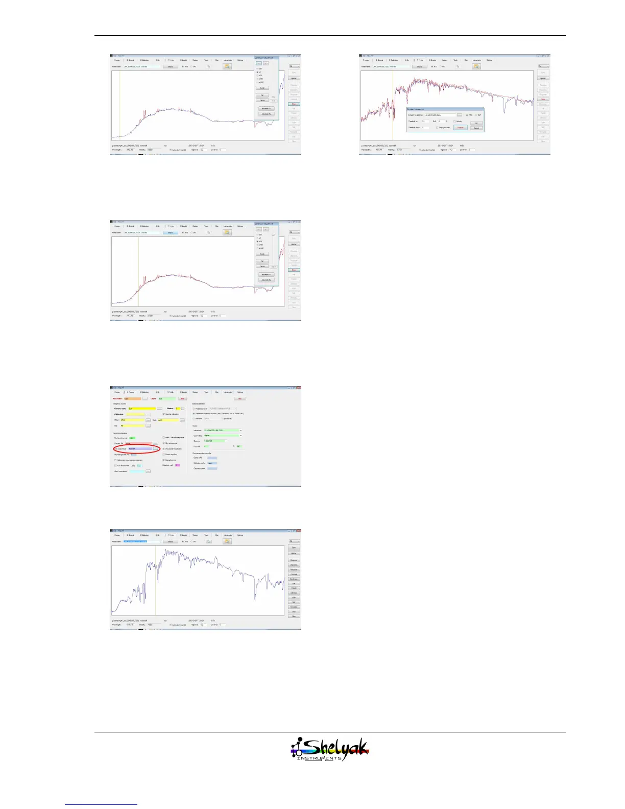
Now, move the cursor in the continuum panel to
smooth the profile, and remove all the noise in the
profile:
Click on OK, and save this response curve.
Now go back to the “2. General” tab, and fill in the
“response curve” field.
You can then re-run, for the third and last time:
This is the actual spectrum of the Sun !
You can compare it with the G2V theoretical spec-
trum (click on the “compare” button):
You can see that the result is excellent - much of the
detail that we could suspect to be noise is in fact the
sunlight signal.
Summary
The spectrum of the Sun is now fully processed.
To do it, you’ve run the data reduction process three
times: the first time to get the raw profile, the sec-
ond one to include the wavelength calibration, and
the last one to correct for the instrumental response
curve. This process needs to be done only once per ob-
serving session. When you observe several objects in
the same night, you can reuse the calibration and the
response curve - to the first order, you can consider
that it only depends on the instrument, and not on
the observing conditions (this may be a little bit more
complex if you need a very accurate measurement).
We invite you to observe many spectra with this
setup and run the data reduction process for each of
them. For a new object, the only point to change is the
input file and the source name in the tab “2. General”
- and run the process in the “4. Go” tab. It takes only
a few seconds.
25