Marsh-McBirney Flo-Mate 2000 - Method; 2-D Method; 2-D Method Alternate

To Next Page

To Previous Page

1-4

.4 Method

A simplified version of the .2, .4, .8 method is to measure the velocity at the .4 position and use this

as . This method is probably the least accurate because it uses only one data point and assumes

that a logarithmic profile exists. This is also called the 60% of depth method.

2-D Method

• Locate the center line of the flow.

• Locate vertical velocity lines (VVL) halfway between the

center line and the side walls of the conduit. This is measured

at the widest part of the flow.

• Take at least seven velocity measurements at different depths

along the center line.

• Take velocity readings at different depths on the VVL. The

distance between these depths should be the same as those on

the center line.

• Take final point velocity readings at the right and left corners of the flow.

• Check the data for any outliers. If a best fit curve of the velocity profile were plotted, an outlier

would lie outside the best fit curve region. See Figure 3-1 on Page 3-2.

• Average all measurements except outliers for . Remember to include the corner measurements.

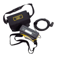
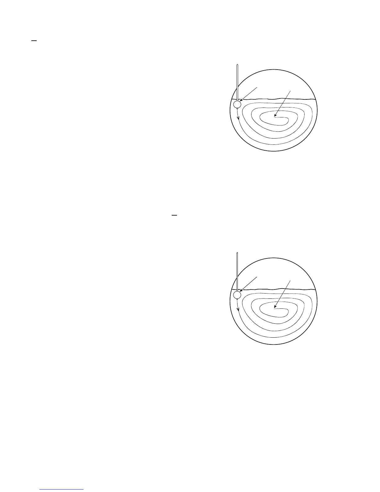
2-D Method Alternate

Another way to do the 2-D profile is with the FPA (fixed point

average) feature of the Model 2000 Flo-Mate. The Flo-Mate

sensor is moved at a constant velocity in a pattern across the flow

that covers the cross-sectional area. The velocity displayed by the

Flo-Mate at the end of the FPA period is the mean velocity.

Comment:

It may take several attempts to get the FPA time set so that the end

of the FPA period coincides with the end of the sensor motion.

• Set the FPA time to the appropriate number of seconds.

• Place the sensor at the start position and wait for a few sec-

onds.

• Press <ON/C> and start moving the sensor.

START

FINISH

START

FINISH

Figure 1-3. 2-D Velocity

Positions

Figure 1-4. 2-D Method

Alternate