Vernier LabQuest 2 - Page 31

LabQuest
®
2 – User Manual
25
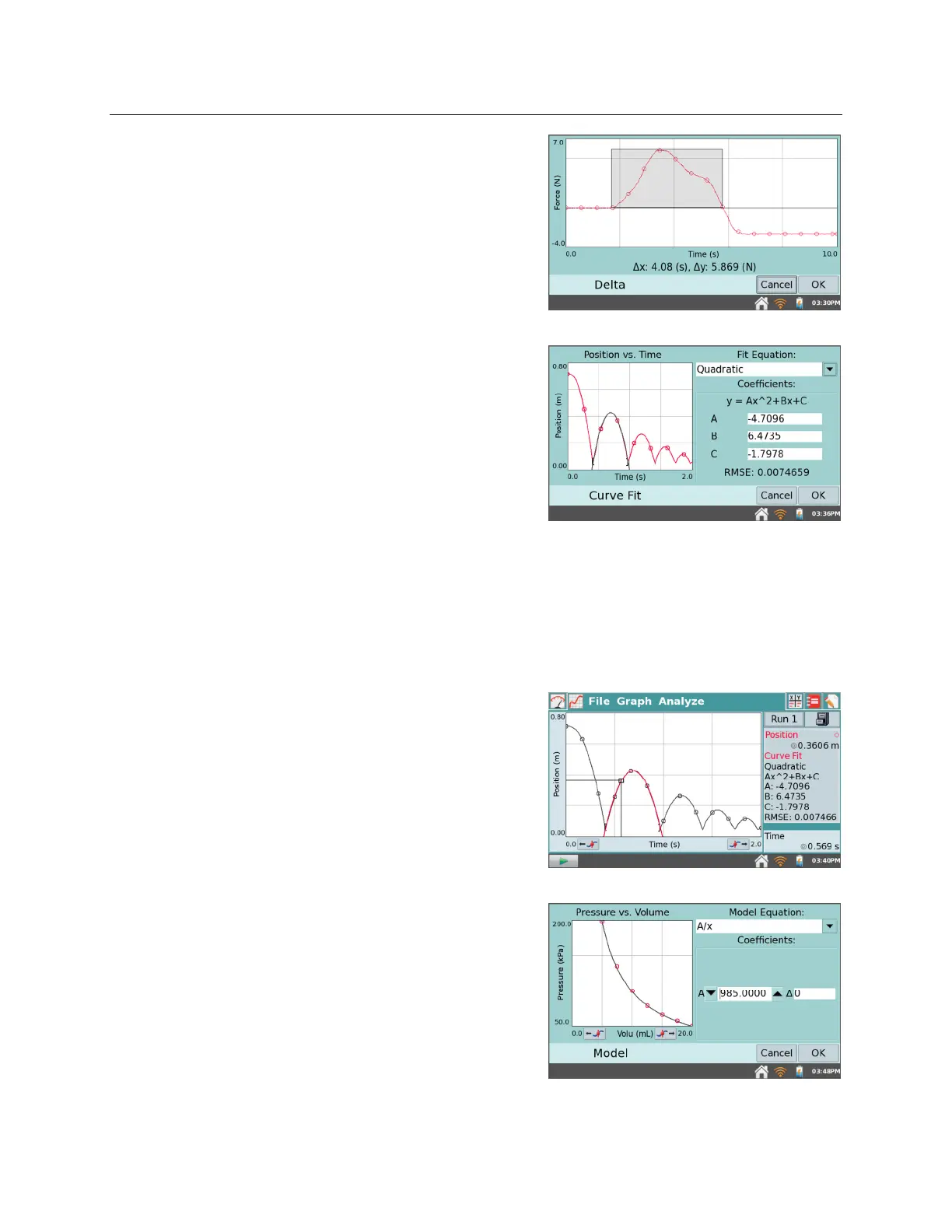
 Delta – The Delta tool opens a preview window
where you can examine x- and y-deltas. Choose
Delta from the Analyze menu to open the preview
window. Then, tap-and-drag to create a box
overlaid on the graph. The vertical side of the box
yields y, and the horizontal side of the box yields
x. Tap OK to keep these values and display the
box on the Graph screen. To exit the Delta tool
without displaying the box on the Graph screen, tap
Cancel.
 Curve Fit – The Curve Fit tool fits a chosen
function to your data. If a region of the graph is
selected, only that region is used for fitting. If there
is no selection, the entire graph is used.
Choose Curve Fit from the Analyze menu. In the
Choose Fit list, choose the desired equation.
LabQuest displays the fit in the preview graph at
the left. The fit coefficients and Root Mean Square
Error (RMSE) are also displayed.
Tap OK to keep this fit and display the curve on the Graph screen. To exit the Curve Fit tool
without applying the curve, tap Cancel.
TIP! The RMSE (root mean square error) is a measure of how well the fit matches the data.
The smaller the RMSE, the closer the data are to the fitted line. The RMSE has the same
units as the y-axis data.
 Interpolate – Once you have performed a curve fit,
you can use the Interpolate tool to read values from
the fitted function. Choose Interpolate from the
Analyze menu, then tap on the graph. The lines
associated with the Examine cursor now locate a
position on the fitted function. Coordinates along
the fitted line are shown in the panel to the right of
the graph. One way to determine that LabQuest is
in the Interpolation mode is by the square Examine
cursor.
 Model –The Model tool manually fits a chosen
function to your data. Choose Model from the
Analyze menu, then choose the desired model
equation from the Model Equation list. LabQuest
displays the modeled function in the preview graph
at left.
The model parameters (e.g., A, B, and C) are
adjustable. Change them by direct entry or by using
the arrows.