HP 54753A User Manual

Transmission Line Theory Applied to Digital Systems
Transmission Line Design
11-7
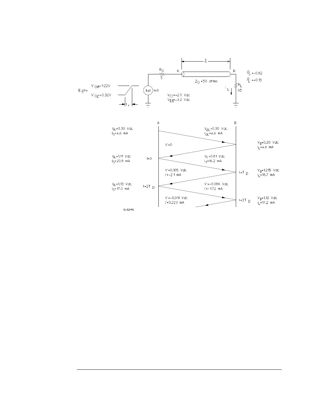
Figure 11-4
Latice Diagram for a Typical Reflection Example
The load resistor is arbitrarily chosen to be 30 percent greater (65 Ω) than the
characteristic impedance (50 Ω) so that reflections will occur. The resulting
reflection coefficient at the load is ρ
L
= + 0.13. Two vertical lines are drawn to
represent the input of the line, point A, and the output of the line, point B. A
line is drawn from point A to point B before
t
= 0 to represent the steady state
conditions. Note that for V
CC
= 2 V and V
EE
= - 3.2 V, the nominal logic levels
are approximately logic 0 = 0.3 V, and logic 1 = 1.14 V. (These power supply
conditions are used to permit convenient measurements when output resistors
are returned directly to ground). For steady state conditions, the line looks like
a short line with a resistance equal to
R
dc
. It can be assumed that
R
dc
is
negligible for this example.

HP 54753A Specifications

General

Brand	HP
Model	54753A
Category	Control Unit
Language	English