This difficulty is overcome by using the
normal time base of the scope for horizontal
deflection, rather than the GCV output. Since
this deflection signal is always linear with
respect to time, then the true nature of the
sweep (linear or log) is displayed. Drawbacks
are a somewhat more difficult determination
of exact frequency points on the scope, and,
depending on the generator, a possible rever-
sal of display from the method used earlier.
Procedure
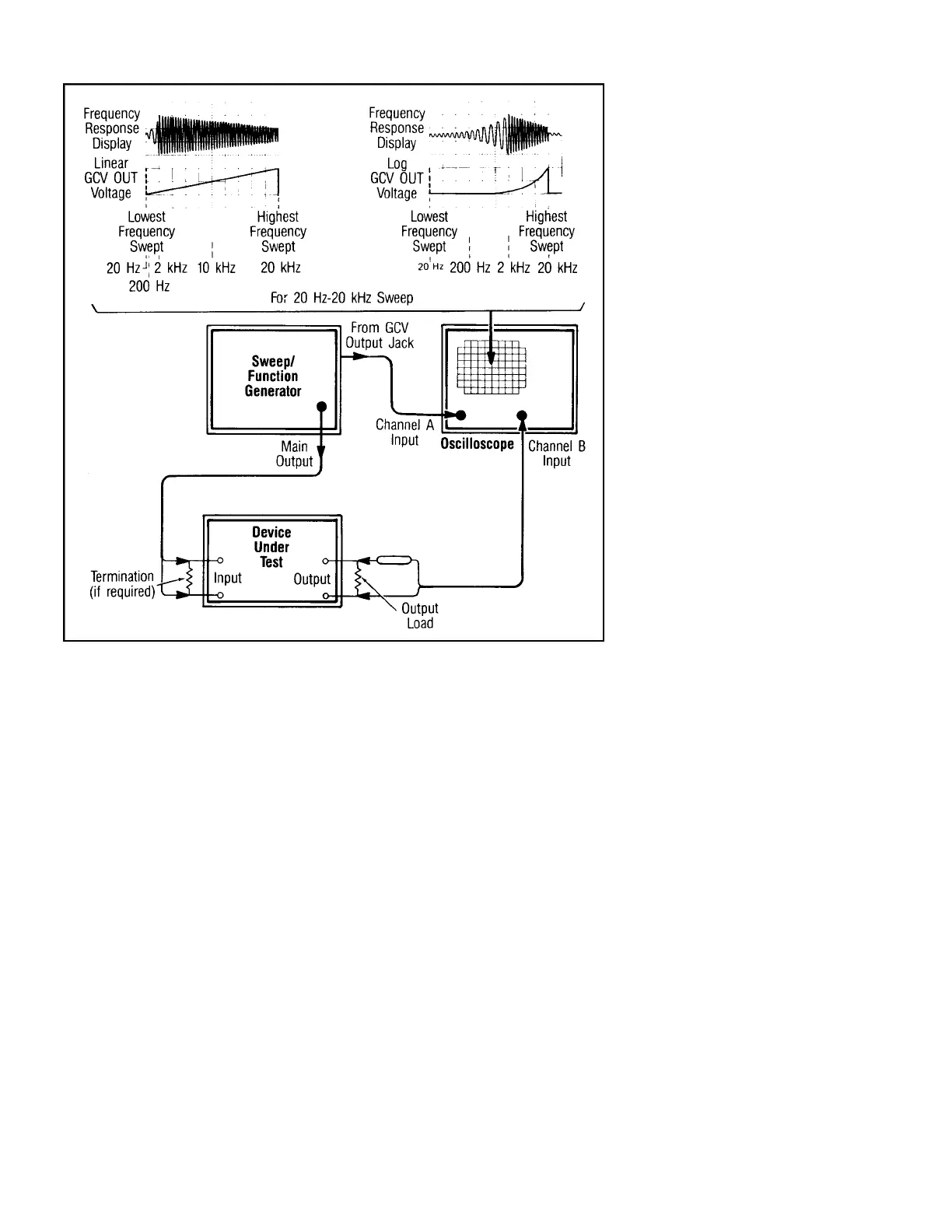
Refer to Fig. 12.
1. Connect the GCV output of the generator
to a vertical input of the oscilloscope, as
shown in the figure. Though not used for
horizontal deflection, the GCV output is
nevertheless useful in setting and deter-
mining frequency points on the display.
2. Select the desired frequency range on the
generator.
3. Set the generator for continuous run
mode, and set the frequency dial for the
desired starting frequency of the sweep.
4. Use DC coupling for the scope input to
which the GCV output is connected.
Initially, select only that channel and
adjust the scope controls to display a flat
trace. Use automatic sync on triggered
sweep scopes.
5. Use the oscilloscope vertical position
control to locate the trace at a convenient
vertical reference point. Note: if the GCV
voltage increases with increased frequen-
cy, the trace should be located near the
bottom of the screen; otherwise, locate it
close to the top. Check the manufactur-
er’s manual for the particular generator.
6. Now set the generator to run at the
desired ending frequency of the sweep.
Without readjusting the vertical position
control, adjust the vertical gain controls
of the oscilloscope (step and vernier) so
that the new trace is located at a conve-
nient point vertically opposite the point
used in step 5.
7. Repeat steps 3, 5, and 6 as required to
attain the two desired vertical positions
for start and stop references.
NOTE
Some generators have separate start frequen-
cy and stop frequency controls, which facili-
tate setting of sweep endpoints. However, the
procedure of steps 3, 5, and 6 is still advis-
able. Moreover, on some units, these controls
are uncalibrated during logarithmic sweeps.
In that case, the procedure is still necessary.
8. Return the frequency dial on the genera-
tor to the sweep starting frequency, and
turn the sweep mode on, selecting linear
or log sweep as desired.
9. Initially, set the sweep rate so that it is
high enough for one or more cycles of
sawtooth waveform to be displayed,
either linear or log, like the bottom traces
in Fig. 12. Set the oscilloscope to trigger
on the GCV waveform (channel A in this
example). Note: direction of the ramp
depends on the particular generator.
10. Adjust the sweep width so that the saw-
tooth ramps between the two screen posi-
tions chosen in steps 5 and 6. The gener-
ator is now sweeping between the two
desired frequencies.
11. Adjust the sweep rate to attain the desired
repetition rate. For viewing convenience,
the highest possible setting is desirable.
However, it must be set low enough to
obtain a few cycles at the lowest frequen-
cies being swept.
12. Readjust the oscilloscope sweep speed to
display one cycle of the sweep voltage
waveform, and spread it out over some
convenient number of horizontal divi-
sions. Each division can later serve as a
frequency marker if the corresponding
frequency is calculated. For example, the
first display in Fig. 12 shows a 20 Hz to
20 kHz linear sweep display spread over
10 divisions. The difference between the
lowest and highest frequency is almost 20
kHz. Therefore, starting from the left of
the display at 20 Hz, each division equals
a frequency increase of 2 kHz. When log
display is used, markers between the low-
est and highest frequencies must be
scaled logarithmically. The second dis-
play in Fig. 12 shows a 1000:1 log sweep
display spread over nine horizontal divi-
sions. Each three divisions equals a
decade of frequency change; that is, after
three divisions, the frequency has
increased one decade or 10:1 (from 20 Hz
to 200 Hz), after six divisions it has
increased another decade or 100:1 (to 2
kHz), and after nine divisions, another
decade, or 1000:1 (to 20 kHz).
APPLICATIONS
Fig. 12 Frequency response measurement, linear/log display method.
12