Chapter 5: Differential Equation Graph Application 123
Setting Description
Solution Dir.
A solution curve is graphed starting at the initial condition value
t0 and continues until
it reaches a target value, which can be either tmin or tmax. The solution direction
determines the target values. Forward will graph the solution curve from
t0 to tmax.
Backward will graph the solution curve from t0 to tmin. Both will graph the solution curve
from
t0 to tmin, and then t0 to tmax.
Independent Assignment of the independent variable for differential equations
1st-order, Nth-order:
x or t
2nd-order: t (fixed)
t0 (or x0) If the independent variable is different from the x-axis variable, you can enter the initial
value for the independent variable (2nd-order and Nth-order only).
tmin (or xmin),
tmax (or xmax)
If the independent variable is different from the x-axis variable, you can enter the
minimum/maximum value for the independent variable (2nd-order and Nth-order only).
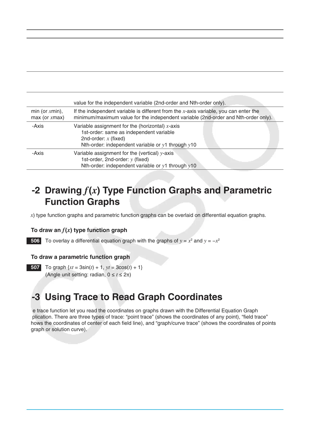
x-Axis Variable assignment for the (horizontal) x-axis
1st-order: same as independent variable
2nd-order: x (fixed)
Nth-order: independent variable or y1 through y10
y-Axis Variable assignment for the (vertical) y-axis
1st-order, 2nd-order: y (fixed)
Nth-order: independent variable or y1 through y10
5-2 Drawing f ( x) Type Function Graphs and Parametric
Function Graphs
f ( x) type function graphs and parametric function graphs can be overlaid on differential equation graphs.
u To draw an f ( x) type function graph
0506 To overlay a differential equation graph with the graphs of y = x
2
and y = −x
2
u To draw a parametric function graph
0507 To graph {xt = 3sin(t) + 1, yt = 3cos(t) + 1}
(Angle unit setting: radian, 0 s t s 2π)
5-3 Using Trace to Read Graph Coordinates
The trace function let you read the coordinates on graphs drawn with the Differential Equation Graph
application. There are three types of trace: “point trace” (shows the coordinates of any point), “field trace”
(shows the coordinates of center of each field line), and “graph/curve trace” (shows the coordinates of points on
a graph or solution curve).
u To start a point trace
On the Differential Equation Graph window, tap K.
u To start a field trace
Draw a slope field (see page 119) or a phase plane (see page 120), and then tap L.