Casio fx-CP400 - Page 133

Chapter 7: Statistics Application 133
k Regression graphs
Regression graphs of each of the paired-variable data can be drawn according to the model formulas under
“Regression types” below.
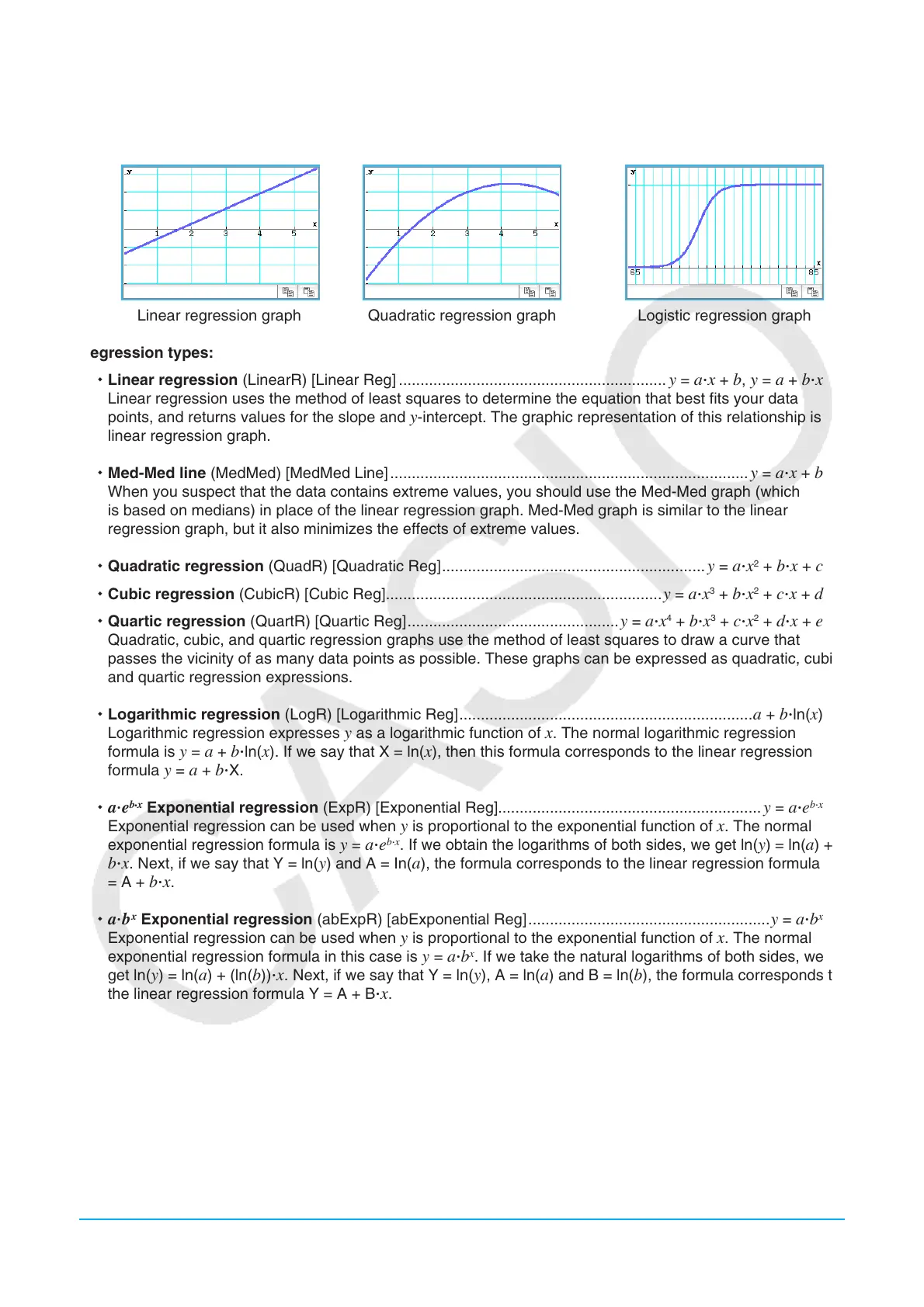
Linear regression graph Quadratic regression graph Logistic regression graph
Regression types:
 Linear regression (LinearR) [Linear Reg] ..............................................................
y = aⴢx + b, y = a + bⴢx
Linear regression uses the method of least squares to determine the equation that best fits your data
points, and returns values for the slope and y-intercept. The graphic representation of this relationship is a
linear regression graph.
 Med-Med line (MedMed) [MedMed Line] ...................................................................................
y = aⴢx + b
When you suspect that the data contains extreme values, you should use the Med-Med graph (which
is based on medians) in place of the linear regression graph. Med-Med graph is similar to the linear
regression graph, but it also minimizes the effects of extreme values.
 Quadratic regression (QuadR) [Quadratic Reg] .............................................................
y = aⴢx
2
+ bⴢx + c
 Cubic regression (CubicR) [Cubic Reg] ................................................................y = aⴢx
3
+ bⴢx
2
+ cⴢx + d
 Quartic regression (QuartR) [Quartic Reg] .................................................y = aⴢx
4
+ bⴢx
3
+ cⴢx
2
+ dⴢx + e
Quadratic, cubic, and quartic regression graphs use the method of least squares to draw a curve that
passes the vicinity of as many data points as possible. These graphs can be expressed as quadratic, cubic,
and quartic regression expressions.
 Logarithmic regression (LogR) [Logarithmic Reg] ....................................................................
a + bⴢln(x)
Logarithmic regression expresses y as a logarithmic function of x. The normal logarithmic regression
formula is y = a + bⴢln(x). If we say that X = ln(x), then this formula corresponds to the linear regression
formula y = a + bⴢX.

aⴢe
b

x
Exponential regression (ExpR) [Exponential Reg]............................................................. y = aⴢe
b
ⴢ
x
Exponential regression can be used when y is proportional to the exponential function of x. The normal
exponential regression formula is y = aⴢe
b
ⴢ
x
. If we obtain the logarithms of both sides, we get ln(y) = ln(a) +
bⴢx. Next, if we say that Y = ln(y) and A = In(a), the formula corresponds to the linear regression formula Y
= A + bⴢx.

aⴢb
x
Exponential regression (abExpR) [abExponential Reg] ........................................................y = aⴢb
x
Exponential regression can be used when y is proportional to the exponential function of x. The normal
exponential regression formula in this case is y = aⴢb
x
. If we take the natural logarithms of both sides, we
get ln(y) = ln(a) + (ln(b))ⴢx. Next, if we say that Y = ln(y), A = ln(a) and B = ln(b), the formula corresponds to
the linear regression formula Y = A + Bⴢx.
 Power regression (PowerR) [Power Reg] ......................................................................................
y = aⴢx
b
Power regression can be used when y is proportional to the power of x. The normal power regression
formula is y = aⴢx
b
. If we obtain the logarithms of both sides, we get ln(y) = ln(a) + bⴢln(x). Next, if we say
that X = ln(x), Y = ln(y), and A = ln(a), the formula corresponds to the linear regression formula Y = A + bⴢX.
 Sinusoidal regression (SinR) [Sinusoidal Reg] ........................................................
y = aⴢsin(bⴢx + c) + d
Sinusoidal regression is best for data that repeats at a regular fixed interval over time.