6.9.4.3. Integration period
Calculating demand over a period of time helps avoid any short peak values (typically, transients caused by
starting heavy inductive loads) from affecting the calculation.
The integration period has:
a programmable duration - in discrete (sub multiples of 60) steps from 1 minute to 60 minutes
two modes of operation:
Fixed (or block mode)
Sliding
The meter applies the selected integration period mode and duration value across all demand channels.
During the integration period a set of rising values are available that represent the currently calculated demand
for each demand channel. These rising values are updated every second by integrating the energy consumed
since the beginning of the period over the total duration of the period.
At the end of each completed integration period (EOI):
the demand calculations are made
if the current demand value is greater than the previous maximum demand value recorded, the new value is
time stamped and replaces the previous maximum
the current demand registers are set to zero
the EOI time-stamping is carried out and a new integration period is started
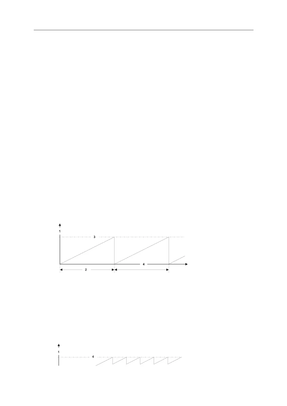
Fixed or block mode
In the fixed or block mode the integration periods have a single predefined duration value.
The illustration below shows two successive fixed or block integration periods with, for example, a duration of 15
minutes. The rising demand value is based on a constant load:
Integration period duration
Sliding mode
In the sliding mode the demand period is divided into between 1 and 15 fixed integration periods. The total
maximum duration of a sliding demand period is 15 (maximum periods) x 60 (maximum minutes) = 900 minutes.
The illustration below shows a sliding mode demand period comprising 4 integration periods with, for example a
duration of T = 5 minutes. The sliding demand period total duration = 20 minutes with the rising demand value
based on a constant load: