kajaaniMCA
i
– Installation, Operating & Service - 9.5 - W4610201 V2.5 EN
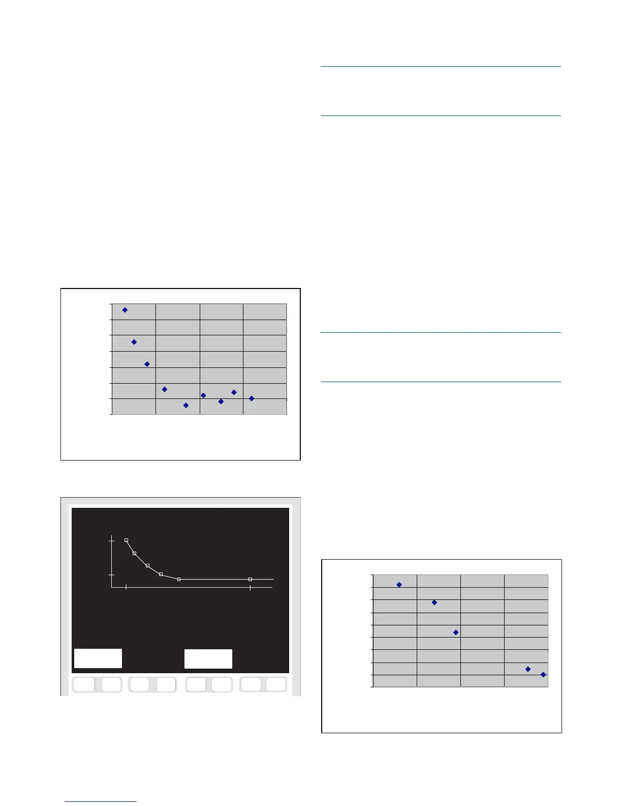
Example 1.
The normal process temperature is 40...50°C
(104...122°F) but drops temporarily to 20°C (68°F)
when the process is started up. The graph (MCAi – Lab
Cs vs. Temperature) shown in Fig. 9.8 was drawn by
using laboratory samples taken while the process was
being started. This graph shows that when the temper-
ature gets below 30°C (86°F) it has an effect on the
MCA
i
measurement. Enter the graph as the correction
curve as follows:
1. Go from M
AIN MENU => SELFDIAGNOSTICS => SPE-
CIAL FUNCTIONS => TEMPERATURE COMPENSATION CURVE
(Fig. 9.9).
2. Choose max. 6 point pairs (Temp. / MCAi – Lab.
Cs) from the curve, at regular temperature intervals.
3. Press [F1&F2] E
DIT and type the point pair values in
fields “T” and “MCAi – Lab” below the graph.
-0.05
0
0.05
0.1
0.15
0.2
0.25
0.3
15 25 35 45 55
Temp. (°C)
MCAi - Lab (%)
Fig. 9.8. Effect of temperature on consistency error.
F7
F6
F5
F4
F8
F3
F1
F2
F9
F10
F11
F12
F13
F14
F15 F16
i
Fig. 9.9. “Temperature compensation curve” display.
Temperature compensation curve
View
0.28 %
-0.02 %
17.00 °C 47.00 °C
T MCA-Lab T MCA-Lab
17.0 °C= 0.28 % 32.0 °C=-0.02 %
20.0 °C= 0.18 % 40.0 °C=-0.01 %
27.0 °C= 0.03 % 47.0 °C=-0.01 %
Edit History
-0.15
-0.1
-0.05
0
0.05
0.1
0.15
0.2
0.25
0.3
17 19 21 23 25
Temp. (°C)
MCAi - Lab (%)
Fig. 9.10. Effect of temperature on consistency error.
NOTE: Make sure that you use the same “MCAi – Lab”
value for the last two points! Otherwise the correction
curve will continue using the slope between the last two
points.
4. If required, press [F5&F6] PREVIEW to see the result-
ing curve before storing it.
5. Press [F3&F4] S
TORE, and you will still be prompted
to confirm the changes. Accept with YES, and the
MCAi will draw the correction curve and take it into
use.
Example 2.
The process temperature is in the range 20...25°C
(68...77°F), and thus errors in the temperature compen-
sation can be expected. The obtained “MCAi – Lab. Cs
vs. Temperature” curve, based on laboratory results, is
shown in Fig. 9.10.
In this case two points are sufficient to determine the
temperature effect. Use for example the points 20°C =
0.2% and 25°C = -0.1%, and enter them to the sensor as
described in the previous example.
NOTE: Make sure that you use the same “MCAi – Lab”
value for the last two points! Otherwise the correction
curve will continue using the slope between the last two
points.
9.C.2. Adjusting the compensation curve
To change the temperature compensation, press [F1&F2]
E
DIT to edit the existing curve. In this mode you can edit
the existing values, add new point pairs (max. 6 pairs),
or delete a point by setting its temperature and MCAi –
Lab values to zero.
9.C.3. History
In the “Temperature compensation curve” display press
[F5&F6] H
ISTORY to view compensation curves used
earlier. Scroll with keys [F1&F2] N
EXT and [F3&F4]
P
REVIOUS.
 Loading...