PicoQuant GmbH HydraHarp 400 Software V. 3.0.0.1
2.2. Timing Resolution
The most critical component in terms of timing resolution in TCSPC measurements will usually be the detector.
However, as opposed to analog transient recording, the time resolution of TCSPC is not limited by the pulse
response of the detector. Only the timing accuracy of registering a photon determines the resolution. The
timing accuracy is limited by the timing uncertainty that the detector introduces in the conversion from a photon
to an electrical pulse. This timing error or uncertainty can be as much as ten times smaller than the detector's
pulse response. The timing uncertainties are usually quantified by specifying the rms error (standard deviation)
or the Full Width Half Maximum (FWHM) of the timing distribution or instrument response function (IRF). Note
that these two notations are related but not identical. Good, but also very expensive detectors, notably Micro
Channel Plate PMTs, can achieve timing uncertainties as small as 25 ps FWHM. Lower cost PMTs or SPADs
may introduce uncertainties of 50 to 500 ps FWHM.
The second most critical source of IRF broadening in fluorescence lifetime measurements with TCSPC is
usually the excitation source. While many laser sources can provide sufficiently short pulses, it is also
necessary to obtain an electrical timing reference signal (sync) for comparison with the fluorescence photon
signal. The type of sync signal available depends on the excitation source. With gain switched diode lasers
(e.g. PDL 800–B) a low jitter electrical sync signal is readily available. The sync signal used here is typically a
narrow negative pulse of −800 mV into 50 Ω (NIM standard). The sharp falling edge is synchronous with the
laser pulse (<3 ps rms jitter for the PDL 800–B). With other lasers (e.g. Ti:Sa) a second detector must be used
to derive a sync signal from the optical pulse train. This is commonly done with a fast photo diode (APD or PIN
diode). The light for this reference detector must be derived from the excitation laser beam e.g. by means of a
semi–transparent mirror. The reference detector must be chosen and set up carefully as it also contributes to
the overall timing error.
Another source of timing error is the timing jitter of the electronic components used for TCSPC. This is caused
by the finite rise / fall–time of the electrical signals used for the time measurement. At the trigger point of
comparators, logic gates etc., the amplitude noise (thermal noise, interference etc.) always present in these
signals is transformed to a corresponding timing error (phase noise). However, the contribution of the
electronics to the total timing error is usually small. For the HydraHarp it is typically 10 ps. Finally, it is always a
good idea to keep electrical noise pick-up low. This is why signal leads should be properly shielded coax
cables, and strong sources of electromagnetic interference should be kept away from the TCSPC detector and
electronics.
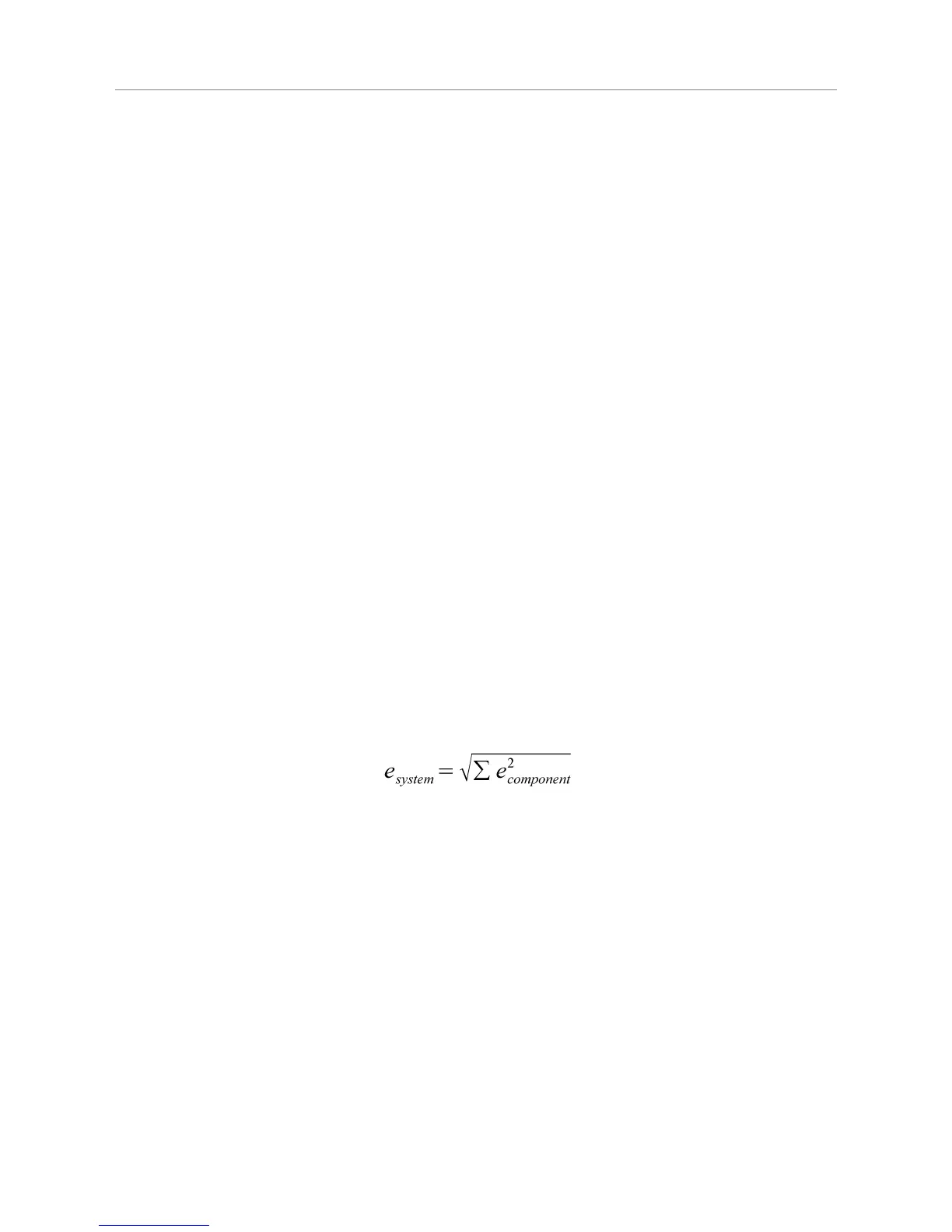
The contribution of the time spread introduced by the individual components of a TCSPC system to the total
IRF strongly depends on their relative magnitude. Strictly, the overall IRF is the convolution of all component
IRFs. An estimate of the overall IRF width, assuming independent noise sources, can be obtained from the
geometric sum of the individual components as an rms figure according to statistical error propagation laws:
Due to the squares in the sum, the total will be dominated by the largest component. It is therefore of little value
to improve a component that is already relatively good. If e.g. the detector has an IRF width of 200 ps FWHM,
shortening the laser pulse from 50 ps to 40 ps is practically of no effect. However, it is difficult to specify a
general lower limit on the fluorescence lifetime that can be measured by a given TCSPC instrument. In addition
to the instrument response function and noise, factors such as quantum yield, fluorophore concentration, and
decay kinetics will affect the measurement. However, as a limit, one can assume that under favourable
conditions lifetimes down to 1/10 of the IRF width (FWHM) can still be recovered via deconvolution.
A final time–resolution related issue worth noting is the channel width of the TCSPC histogram. As outlined
above, the analog electronic processing of the timing signals (detector, amplifiers, CFD etc.) creates a
continuous distribution around any true time value. In order to form a histogram, at some point the timing
results must be quantized. This is done by an Analog to Digital Converter (ADC) or an integrated Time–to–
Digital Converter (TDC). This quantization introduces another random error, if chosen too coarse. The
quantization step width (i.e. the resolution) must therefore be small compared with the continuous IRF. As a
minimum sampling frequency, from the information theoretical point of view, one would assume the Nyquist
frequency. That is, the signal should be sampled at least at twice the highest frequency contained in it. For
practical purposes one may wish to exceed this limit where possible, but there is usually little benefit in
sampling the histogram at resolutions much higher than 1/10 of the overall IRF width of the analog part of the
system.
Page 8