5120A/5115A Operations and Maintenance Manual 89
phase even if quadrature mixers were employed. Thus analog test sets must be maintained near
quadrature where the sine of the phase is nearly linear and equal to the phase angle. When
measuring sources, the quadrature condition is achieved by a long time constant, phase-lock loop.
Down-conversion is performed on the second input channel, and the two are subtracted to obtain
the phase difference between the two sources. However, if the two input signals have different
nominal frequencies, then the phase of the second channel must be scaled to the same nominal
frequency as the first channel. For example, if we were calculating the phase difference between a
10 MHz signal and a 5 MHz signal, then the phase difference between the 5 MHz source and the
LO must be multiplied by 2 before subtraction from the phase difference of the 10 MHz signal and
its LO. The subtraction process causes the phase noise of the instrument’s clock oscillator to
cancel, just as it does in a dual-mixer, phase-difference, measurement system.
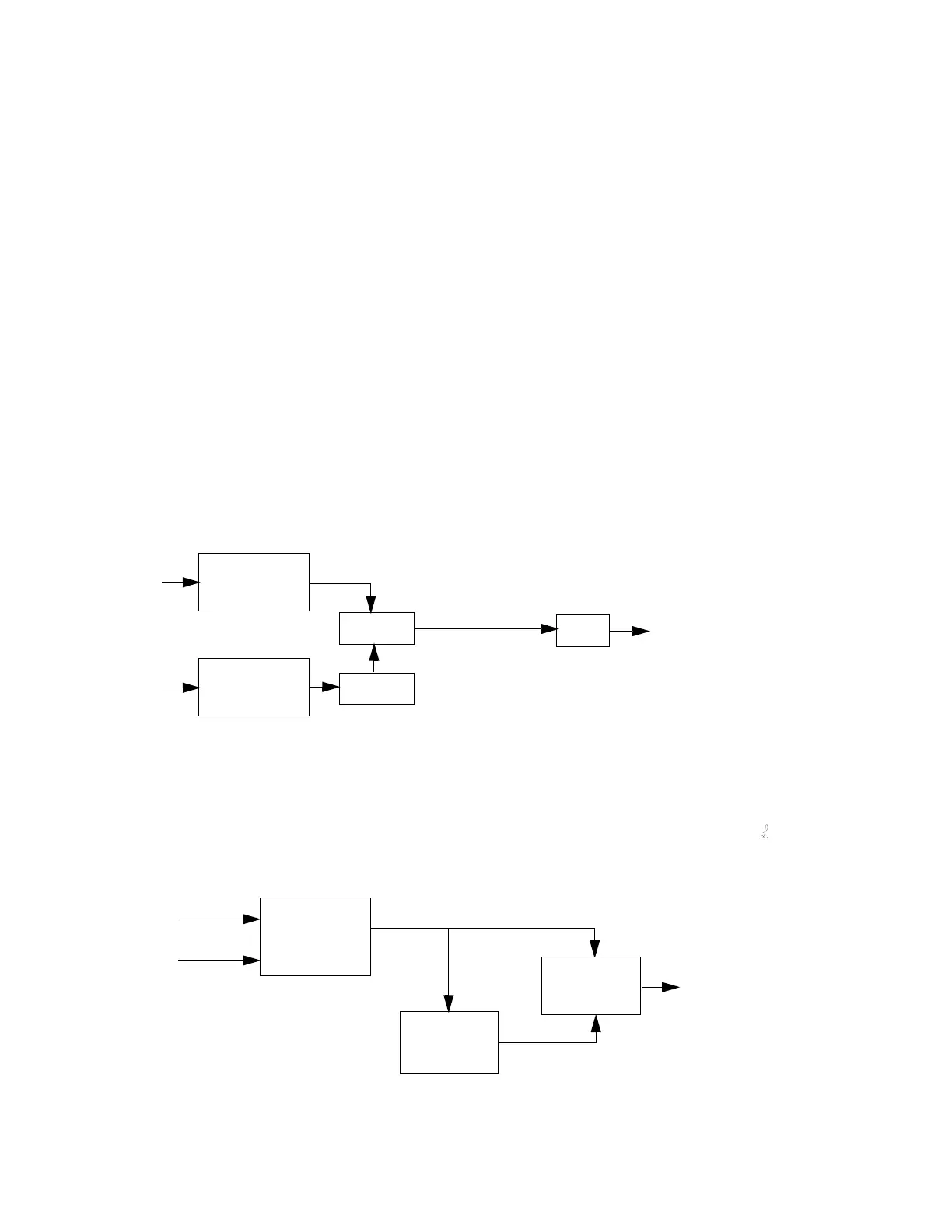
The frequency content of the measured phase difference is analyzed by computing the Discrete
Fourier Transform (DFT) of the phase difference. The computation to this point is shown in
Figure B-4. However, if the Power Spectral Density (PSD) of the phase were computed from the
DFT, the broadband noise floor would be limited by the white noise of the ADCs at a level of –150
dBc/Hz or worse with today’s best converters. This is the price that has been paid for the
convenience of operation without a PLL or need for calibration and would make the direct-digital
approach uninteresting for measuring precision oscillators, except for the fact that convenient
methods exist to overcome the limitation.
Figure B-4: Sample, Down-convert and Transform: After down-conversion, the phase differences are scaled,
subtracted, and Fourier analyzed to determine the frequency content.
The power spectral density of phase, S
φ
(f,) is the squared magnitude of the Fourier transform. This
computation is performed by the 5115A as shown in Figure 5. The instrument displays
(f), which
is defined to be equal to half the spectral density.
Figure B-5: 5115A: The power spectral density of the phase is computed by multiplying the phase by its complex
conjugate and averaging
Φ
1
Φ
CLK
Φ
ADC1
+–
Sample and
Down Convert
Input 1
Input 2
Subtract
Scale
DFT
Φ
∗
2
Φ
∗
CLK
Φ
∗
ADC2
+–
Φ
1
Φ
2
Φ
ADC1
Φ
ADC2
–+–
Sample and
Down-convert
Φ
1
Φ
2
Φ
ADC1
Φ
ADC
–+–
Φ
2
Φ
∗
2
ω
1
ω
------
2
=
Sample,
Down-convert,
& Transform
Input 1
Reference 2
Complex
Conjugate
Φ
∗
1
Φ
∗
2
Φ
∗
ADC1
Φ
∗
ADC2
–+–
S
Φ
1
Φ
2
–
f() 2L f()=
Multiply and
Average
Φ
1
Φ
2
Φ
ADC1
Φ
ADC2
–+–
 Loading...