04/03 347 LB 444
43
If the product is very inhomogeneous, take several samples in quick succession and cal-
culate an average value from their density or concentration values.
Stop measurement by pressing the <run> button again.
Accept result with <enter>. Cursor jumps to next row.
Enter the density value of the sample(s) in g/cm
3
determined in the lab and confirm with
<enter>. Cursor jumps to third row.
Push <enter> to confirm current product temperature.
Rates 2. to 10. must all contain “0”. If “0” is already there, scroll through the rates with
<more> until you get to the submenu group Data input / Calculate. Otherwise, delete
values with <clear> and confirm each with <enter>.
Push <sk2> to select Calculate
Select calibration mode “one” = one-point calibration
Push <enter> to confirm the default value for measurement in g/cm
3
or calculate the
absorption coefficients and enter it in Result a1.
Calibration starts as soon as you confirm with <enter>.
Zero count rate I0 is displayed. Continue with <more>.
The entered linear absorption coefficient for this application is displayed. It must not
change during one-point calibration
. If it has changed, at least one more value pair is
available.
Correction:
Delete the additional value pair.
Run through steps 15 – 17 once more.
Push <more> to skip other coefficients.
If necessary, enter a factor for multiplicative correction of the measured values to correct
the gradient of the linear line. This becomes evident only during measurement and is
only required when the absorption coefficient is too small or too big.
If necessary, enter an Offset for additive correction of the measured values to offset the
straight line on the Y-axis.
With TC: display of temperature-corrected density values.
Push <done> to return to submenu group Data / Calculate.
Push <run> to start measurement.
For later changes of the current output limit values, calculate calibration curve once
more, since during calculation of the curve the curve is checked for monotony.
Two- and Multi-Point Calibration
The gradient of the calibration curve can be determined accurately. Select the calibration
mode depending on the number of value pairs.
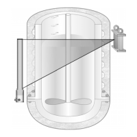
Prerequisite: Pipeline or container must be filled completely.
Push <more> to select menu group Calibrate / Live Display.
Push <sk1> to call the Calibrate submenu.
Select product.
Specify if it is a suspension measurement.
Select unit.
Push <sk1> to select the Data input submenu.
Deselect Calibr. Data transfer with “No”
Read in 1. Rate: cursor appears in the row “1. Rate = cps”.
Push <run>. Count rate and temperature (if a temperature sensor is connected) are
read in. Wait until the measuring value has become stable (20 to 50 s). While reading-in
the count rate, the density of the products must not change.
While reading in the count rate, take a sample of the product from the pipeline and de-
termine its density or concentration. If the product is very inhomogeneous, take several
samples in quick succession and calculate an average value from their density or concen-
tration values.