Using a graphic display calculator
© Oxford University Press 2012: this may be reproduced for class use solely for the purchaser’s institute
Casio fx-9860GII
Press
OPTN
F4
CALC |
F3
d
d
2
x
2
to enter the second derivative template.
Enter Y1 in the template as the function using the same procedure to
enter the Y.
Enter the value of x as 0.
Repeat for the second derivative when x = 3.
In this case we are not certain what the nature of the stationary point is
at (0, 0) but the point (3, −27) is a minimum because f ″(x) > 0.
Evaluate f ′(x) either side of x = 0, in this case using x = –0.01 and x = 0.01.
To evaluate the derivatives follow the same steps as before, but use
F2
d
dx
.
The gradient is negative either side of the stationary point.
Hence (0, 0) is a negative point of infl ection.
The graph on the right illustrates the curve, the minimum at (3, –27) and
the point of infl ection at (0, 0).
3 Integral calculus
The calculator can fi nd the values of defi nite integrals either on a calculator page or graphically.
The calculator method is quicker, but the graphical method is clearer and shows
discontinuities, negative areas and other anomalies that can arise.
3.1 Finding the value of a defi nite integral
Example 36
Evaluate
xx
x
−
⎛
⎝
⎜
⎞
⎠
⎟
⌠
⌡
⎮
3
2
8
d
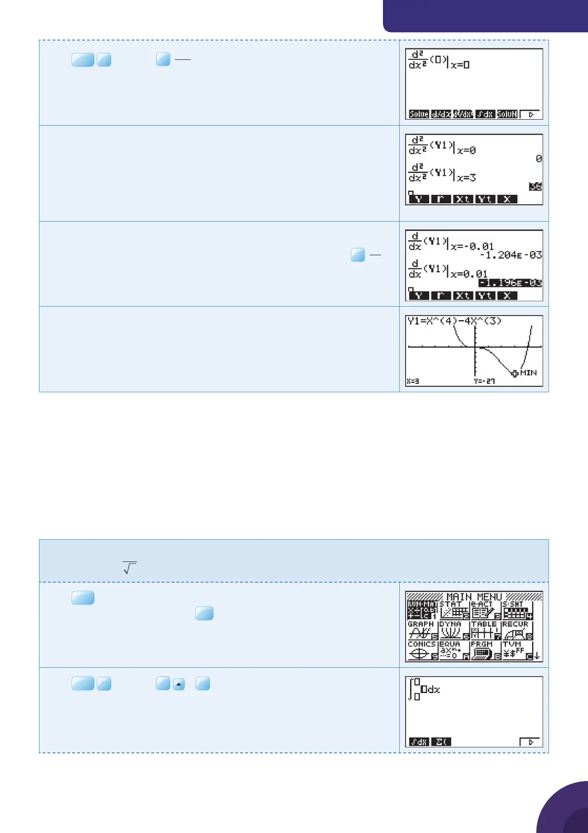
Press
MENU
. You will see the dialog box as shown on the right.
Choose 1: RUN·MAT and press
Press
OPTN
F4
CALC |
F6
|
F1
∫dx to enter the second derivative
template.
In this example you will also use templates to enter the rational function
and the square root.
{ Continued on next page
35

 Loading...