PicoQuant GmbH HydraHarp 400 Software V. 3.0.0.1
The principle of a classical CFD is the comparison of the original detector signal with an amplified, inverted and
delayed version of itself. The signal derived from this comparison changes its polarity exactly when a constant
fraction of the detector pulse height is reached. The zero crossing point of this signal is therefore suitable to
derive a timing signal independent from the amplitude of the input pulse. In practice the comparison is done by
a summation. The timing is done by a subsequent threshold trigger of the sum signal using a settable level, the
so called zero cross trigger. Newer CFD designs achieve the same objective by differentiating the input signal
and triggering on the zero crossing of the differentiated signal. This is the case for the HydraHarp 400. This has
the benefit of adaption to different detector types without a need for changing physical delay lines.
Making the zero cross level adjustable (slightly above zero) allows to adapt to the noise levels in the given
signal, since otherwise an infinitely small signal could trigger the zero cross comparator. Typical CFDs
furthermore permit setting of a discriminator threshold that determines the lower limit the detector pulse
amplitude must pass. This is primarily used to suppress dynode noise from PMTs.
Similar as for the detector signal, the sync signal must be made available to the timing circuitry. Since the sync
pulses are usually of well defined amplitude and shape, a simple settable comparator (level trigger) is often
sufficient to adapt to different sync sources. Nevertheless, it can be valuable to have a CFD also on the sync
channel. A suitably designed CFD is also usable with pre–shaped signals and simply becomes a level trigger in
this case. This is the case also for the HydraHarp 400. Note that the input signals must have sufficiently fast
rise / fall times in the sub-nanosecond to 10 nanosecond range.
The signals from the two input discriminators / triggers are in conventional systems fed to a Time to Amplitude
Converter (TAC). This circuit is essentially a highly linear ramp generator that is started by one signal and
stopped by the other. The result is a voltage proportional to the time difference between the two signals. In
conventional systems the voltage obtained from the TAC is then fed to an Analog to Digital Converter (ADC)
which provides the digital timing value used to address the histogrammer. The ADC must be very fast in order
to keep the dead time of the system short. Furthermore it must guarantee a very good linearity (over the full
range as well as differentially). These are criteria difficult to meet simultaneously, particularly with ADCs of high
resolution (e.g. 12 bits) as is desirable for TCSPC over many histogram channels.
The histogrammer has to increment each histogram memory cell, whose digital address in the histogram
memory it receives from the ADC. This is commonly done by fast digital logic e.g. in the form of Field
Programmable Gate Arrays (FPGA) or a microprocessor. Since the histogram memory must also be available
for data readout, the histogrammer must occasionally stop processing incoming data. This prevents continuous
data collection. Sophisticated TCSPC systems solve this problem by switching between two or more memory
blocks, so that one is always available for incoming data.
While this section so far outlined the typical structure of conventional TCSPC systems, it is worth noting that
the design of the HydraHarp 400 is somewhat different. Today, it is state–of–the–art that the tasks
conventionally performed by TAC and ADC are carried out by a so called Time to Digital Converter (TDC).
These circuits allow not only picosecond timing but can also extend the measurable time span to virtually any
length by means of digital counters. The HydraHarp 400 does not use one such circuit but one for each input
channel and one for the SYNC input. They independently work on each input signal and provide picosecond
arrival times that then can be processed further, with a lot more options than in conventional TCSPC systems.
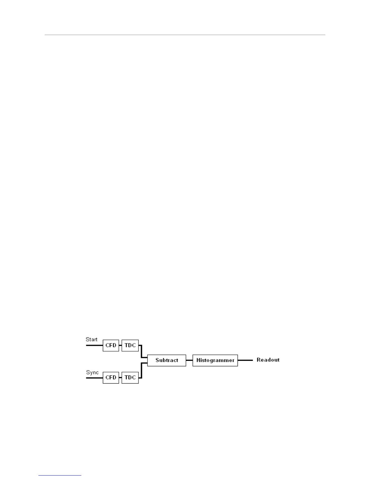
In the case of classical TCSPC, this processing consists of a subtraction of the two time figures and
histogramming of the differences. This is identical to the classical start–stop measurements of the conventional
TAC approach. The following figure exemplifies this for one detector channel (Start).
The full strength of the HydraHarp design is exploited by collecting the unprocessed independent arrival times
as a continuous data stream for more advanced analysis. Details on such advanced analysis can be found in
the literature. In this case the on–board memory is reconfigured as a large data buffer (FIFO) so that count rate
bursts and irregular data transfer are decoupled. This permits uninterrupted continuous data collection with
high throughput. This mode of operation is called Time–Tagged Time–Resolved (TTTR) mode. Details are
described in section 5.3.
Page 11