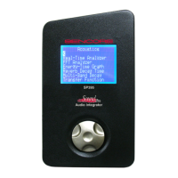
SP395 SoundPro Audio Integrator Form7492 Operation Manual
36
unless Flat is selected. This means that a flat input signal will show up like the A or C
curve, with the lows and highs attenuated accordingly. This can be useful in community
noise studies, to determine what frequency bands may be exceeding a standard referenced
to A or C weighting. You may also select a “Diff” (difference) mode to show the change
in RTA which occurred from a previous RTA captured into memory.
8. Graphed FFT test data – Test data by band showing bar graph levels.
9. Graph Range – dB range of graphed levels. Adjust the dB range as needed so that the
display fits on the vertical axis, by selecting and changing the dB value at the bottom of
the vertical axis.
10. Average SPL – The digital SPL measurement that is displayed along the bottom of the
graph is calculated from an average of the RTA bands and is therefore slightly less
accurate than the standard SPL function. It is provided here for convenience while using
the RTA display. You can select dB SPL – the unweighted full-band SPL level; dBA -
the A-weighted SPL; dBC - the C-weighted SPL. Turn the control knob until the desired
weighting value is displayed, then click to select the new value.
11. Measurement Cursor – Click the control knob on the cursor control field, then turn the
control knob to move the cursor to any measurement bar to read out the exact frequency
and dB level. Cursor measurements can be made in the Run or Pause mode, or on recalled
FFT graphs.
12. Cursor Level – Indicates the level SPL of the cursor position (octave or 1/3 octave band)
on the graph. The measurement Cursor allows you to analyze the FFT graph display in
detail. It is an inverse-highlighted vertical bar that you can position horizontally along the
graph. The center frequency of the selected band and the band's dB SPL level are
displayed in the lower right portion of the graph. Cursor measurements can be made in the
Run or Hold mode, or on recalled FFT graphs. To position the Measurement cursor along
the graph, highlight the frequency "Measurement Cursor" field and click on it
(underlined). Rotate the control knob to move the cursor.
Overlay – Select Flat response (normal), or the A or C-weighting curve. Note that the A or
C overlay filters actually modify the data on the screen. This means that a flat input signal
will show up like the A or C curve, with the lows and highs attenuated accordingly. This
can be useful in community noise studies, to determine what frequency bands may be
exceeding a standard referenced to A or C weighting.
To use the FFT function:
1. Position the microphone. A measurement microphone is normally placed at the desired
measurement location and pointed at the ceiling to be omni directional to all system
loudspeakers. Apply phantom power to the microphone and select the best gain range in
the top toolbar section.
2. (Optional) Connect a constant-level pink noise signal to the audio system. To use the
SP395 as a pink noise signal source, connect a cable from an SP395 output connector to
the desired input on the audio system. There will not be an output from the system until
the FFT and signal generator are turned on from the FFT display. The output level of the
pink noise is adjustable in the Signal Generator bottom toolbar section. Caution: Preset
the amplifier gain to minimum to prevent speaker damage when the FFT test is turned
on.
3. Select the octave band filter resolution. Use 1/6 or 1/12 octave for most FFT analysis,
as this resolution provides the best resolution to discern differences in the audio sub-
octave bands.