Statistics 12-7
8312STAT.DOC TI-83 international English Bob Fedorisko Revised: 02/19/01 12:42 PM Printed: 02/19/01 1:37
PM Page 7 of 38
The residual pattern indicates a curvature associated with this data set for
which the linear model did not account. The residual plot emphasizes a
downward curvature, so a model that curves down with the data would be
more accurate. Perhaps a function such as square root would fit. Try a power
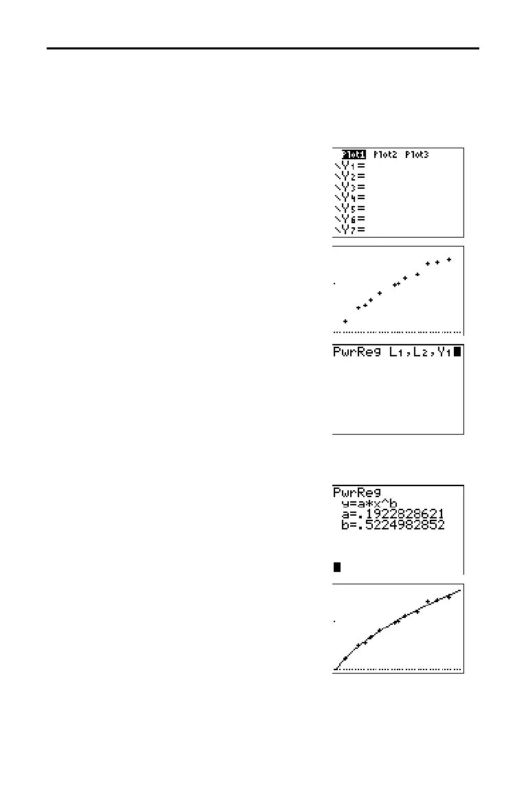
regression to fit a function of the form y = a
ä
x
b
.
22. Press
o
to display the
Y=
editor.
Press
‘
to clear the linear regression
equation from
Y
1
. Press
}
Í
to turn
on plot 1. Press
~
Í
to turn off plot
2.
23. Press
q
9 to select 9:ZoomStat from
the
ZOOM
menu. The window variables
are adjusted automatically, and the
original scatter plot of time-versus-
length data (plot 1) is displayed.
24. Press
…
~
ƒ
[
A
] to select
A:PwrReg from the
STAT CALC
menu.
PwrReg is pasted to the home screen.
Press
y
[
L1
]
¢
y
[
L2
]
¢
. Press
~
1 to display the
VARS Y
.
VARS
FUNCTION
secondary menu, and then
press
1 to select 1:Y
1
. L
1
, L
2
, and Y
1
are
pasted to the home screen as arguments
to
PwrReg.
25. Press
Í
to calculate the power
regression. Values for
a and b are
displayed on the home screen. The
power regression equation is stored in
Y
1
. Residuals are calculated and stored
automatically in the list name
RESID.
26. Press
s
. The regression line and the
scatter plot are displayed.
 Loading...


