Texas Instruments TI-83 - Defining and Displaying Polar Graphs

Polar Graphing 5-3
8305POLR.DOC TI-83 international English Bob Fedorisko Revised: 02/19/01 12:19 PM Printed: 02/19/01 1:36
PM Page 3 of 6
The steps for defining a polar graph are similar to the steps
for defining a function graph. Chapter 5 assumes that you
are familiar with Chapter 3: Function Graphing. Chapter 5
details aspects of polar graphing that differ from function
graphing.
To display the mode screen, press
z
. To graph polar
equations, you must select
Pol graphing mode before you
enter values for the window variables and before you enter
polar equations.
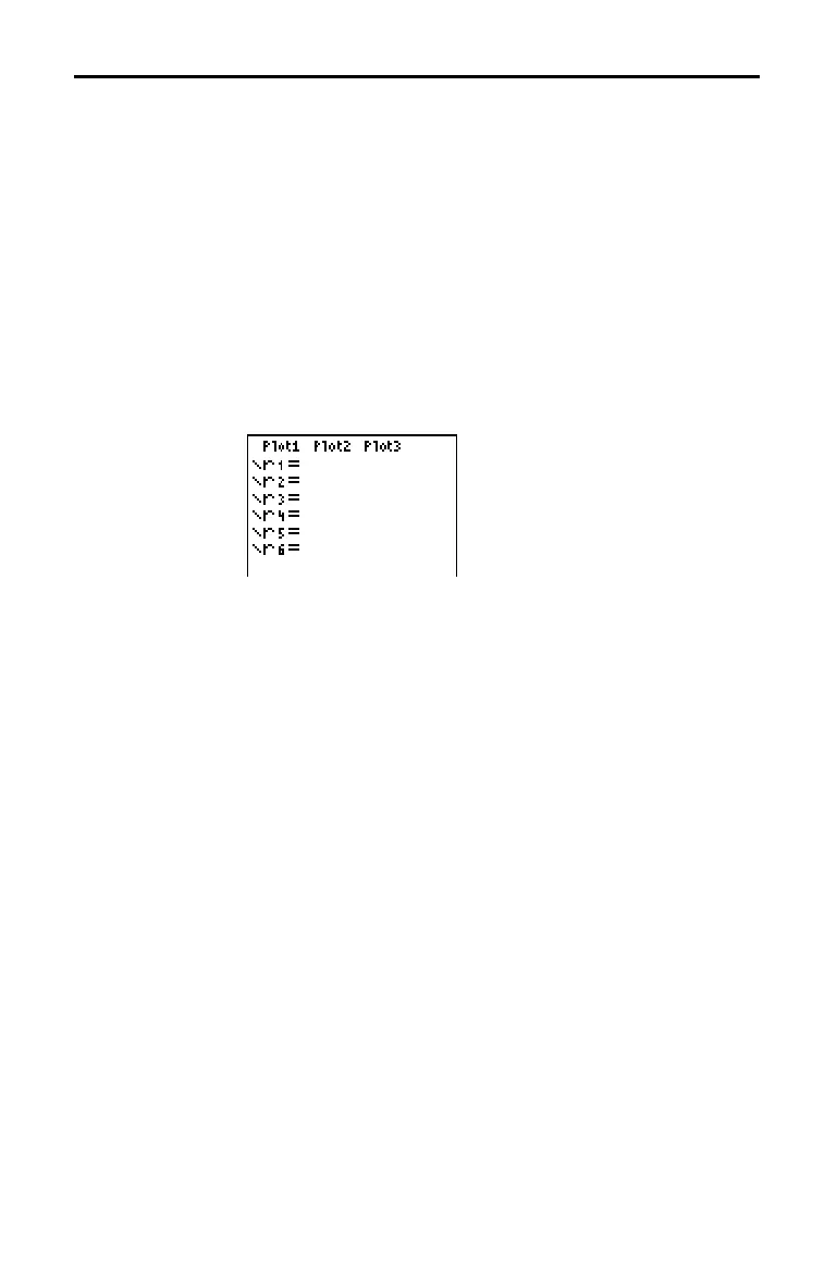
After selecting
Pol graphing mode, press
o
to display the
polar
Y=
editor.
In this editor, you can enter and display up to six polar
equations,
r
1
through r
6
. Each is defined in terms of the
independent variable
q
(page 5
.
4).
The icons to the left of
r
1
through r
6
represent the graph
style of each polar equation (Chapter 3). The default in
Pol
graphing mode is
ç
(line), which connects plotted points.
Line,
è
(thick),
ë
(path),
ì
(animate), and
í
(dot) styles are
available for polar graphing.
Defining and Displaying Polar Graphs
TI-83 Graphing
Mode Similarities
Setting Polar
Graphing Mode
Displaying the
Polar Y= Editor
Selecting Graph
Styles