Texas Instruments TI-83

Inferential Statistics and Distributions 13-29
8313INFE.DOC TI-83 international English Bob Fedorisko Revised: 02/19/01 12:47 PM Printed: 02/19/01 1:38 PM
Page 29 of 36
To display the
DISTR
menu, press
y
[
DISTR
].
DISTR DRAW
1: normalpdf(
Normal probability density
2: normalcdf(
Normal distribution probability
3: invNorm(
Inverse cumulative normal distribution
4: tpdf(
Student-
t
probability density
5: tcdf(
Student-
t
distribution probability
6:
c
2
pdf(
Chi-square probability density
7:
c
2
cdf
Chi-square distribution probability
8:
Ü
pdf( Û
probability density
9:
Ü
cdf( Û
distribution probability
0: binompdf(
Binomial probability
A: binomcdf(
Binomial cumulative density
B: poissonpdf(
Poisson probability
C: poissoncdf(
Poisson cumulative density
D: geometpdf(
Geometric probability
E: geometcdf(
Geometric cumulative density
Note:
L
1
å
99 and 1
å
99 specify infinity. If you want to view the area left
of
upperbound
, for example, specify
lowerbound
=
L
1
å
99.
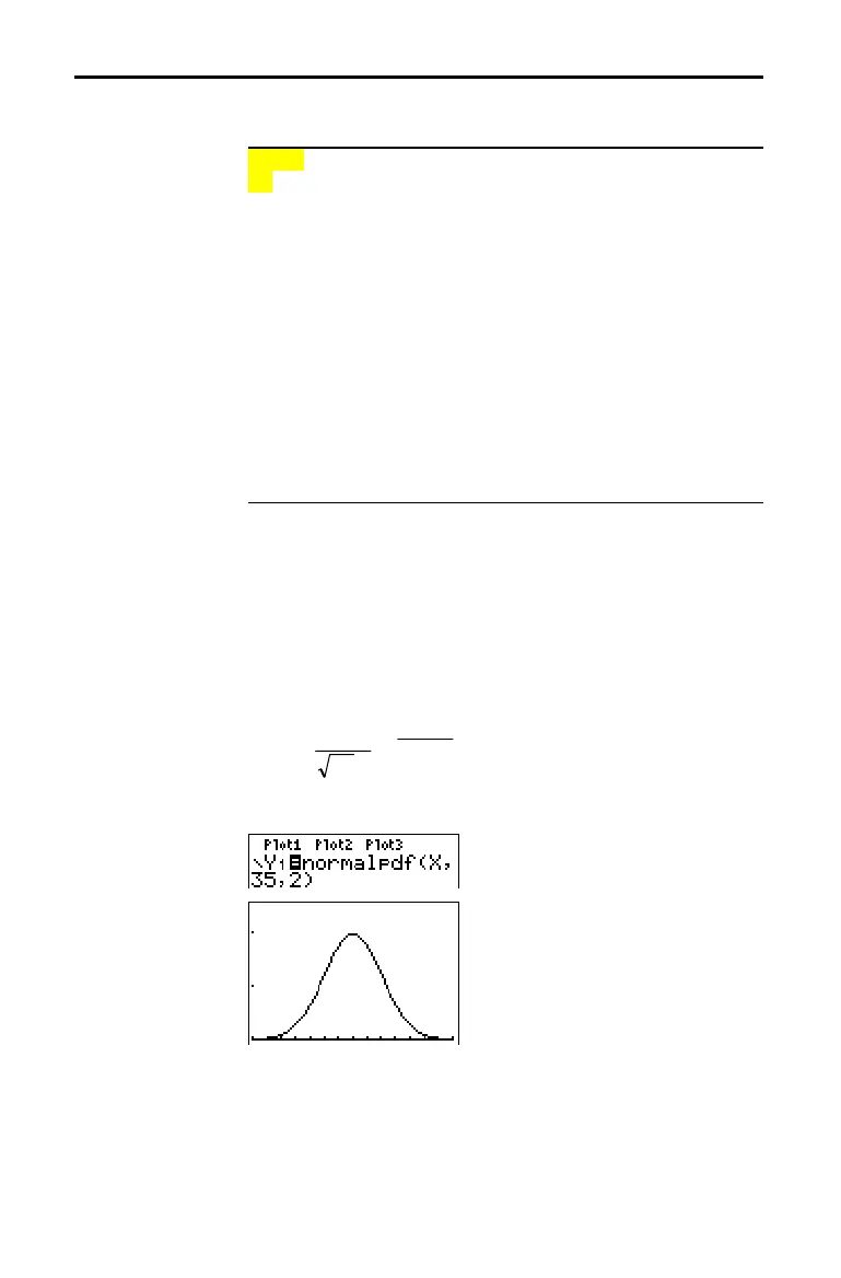
norwmalpdf(
computes the probability density function
(pdf) for the normal distribution at a specified
x
value. The
defaults are mean
m
=0 and standard deviation
s
=1. To plot
the normal distribution, paste
normalpdf(
to the
Y=
editor.
The probability density function (pdf) is:
fx e
x
()
=>
−
−
1
2
0
2
2
2
πσ
σ
µ
σ
()
,
normalpdf(
x
[
,
m
,
s
]
)
Note:
For this example,
Xmin = 28
Xmax = 42
Ymin = 0
Ymax = .25
Tip:
For plotting the normal distribution, you can set window variables
Xmin
and
Xmax
so that the mean
m
falls between them, and then
select
0:ZoomFit
from the
ZOOM
menu.
Distribution Functions
DISTR menu
normalpdf(