20 Chapter 1
Introduction and Measurement Theory
Cable Impedance and Structural Return Loss Measurement Theory
The series may be reduced to a simple form to leave us with the relationship shown
in Equation 10. The term L is a function of the loss of the cable at a specific
frequency and the wavelength at that frequency.
Equation 10
The term (L
2
)/(1−L
2
) can be thought of as the number of bumps that are
contributing to SRL. It represents a balance between the contribution of loss in a
single bump and further bumps in the cable for the specified frequency and cable
loss. Calculate the distance into the cable by multiplying the term (L
2
)/(1−L
2
) by the
distance between bumps.
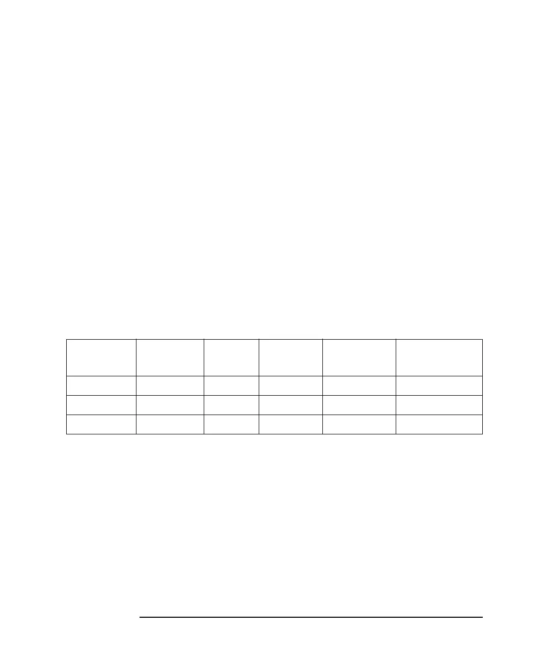
Table 1-1 illustrates some calculated values for a typical trunk cable. From the table,
bumps spaced 1.5 meters apart out to 307 meters will contribute to SRL.
Table 1-1 SRL Equation Constant
How to Use Table 1-1
Refer to Figure 1-2 and Equation 10 for the following discussion.
Γ = the reflection coefficient of each bump (V
reflected
/V
incident
)
L = the cable loss between bumps (V
transmitted
/V
incident
)
The distance between bumps equals λ/2 (1/2 wavelength).
Typical values:
Γ<< 1
L ≤ 1 for low loss cable
SRL
=
Vref
Vin
-----------
= Γ
L
2
1L
2
–
---------------
Frequency
Spacing
(λ/2)m
Loss
(dB)/m
dB/bump
bumps
L
2
/(1−L
2
)
Distance(m)
100 MHz 1.5 0.014 −0.02 205 307
500 MHz 0.3 0.033 −0.01 433 129
1 GHz 0.15 0.05 −0.0075 554 83
 Loading...