HP F2226A - 48GII Graphic Calculator - Page 502

Page 16-24
 Change TYPE to FUNCTION, if needed
 Change EQ to ‘0.5*COS(X)-0.25*SIN(X)+SIN(X-3)*H(X-3)’.
 Make sure that
Indep is set to ‘X’.
 Press @ERASE @DRAW to plot the function.
 Press @EDIT L @LABEL to see the plot.
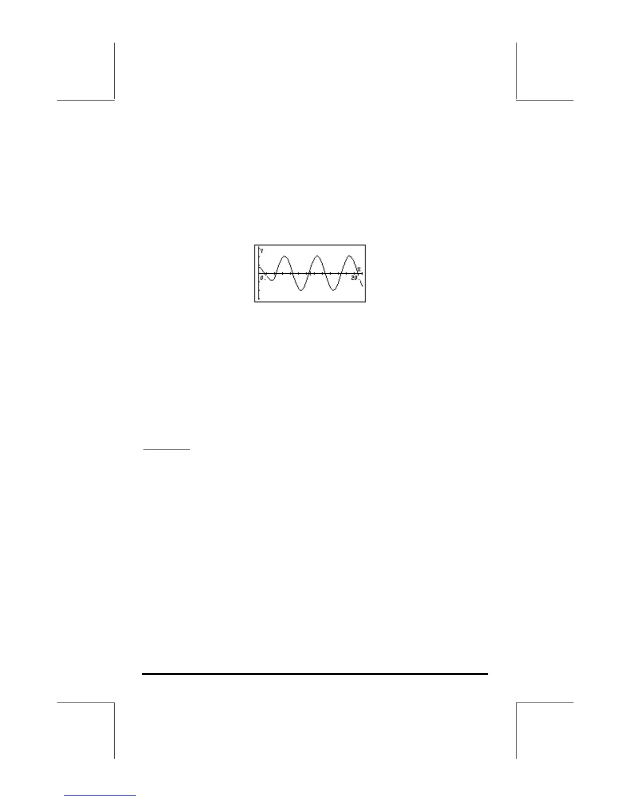
The resulting graph will look like this:
Notice that the signal starts with a relatively small amplitude, but suddenly, at
t=3, it switches to an oscillatory signal with a larger amplitude. The
difference between the behavior of the signal before and after t = 3 is the
“switching on” of the particular solution y
p
(t) = sin(t-3)⋅H(t-3). The behavior of
the signal before t = 3 represents the contribution of the homogeneous
solution, y
h
(t) = y
o
cos t + y
1
sin t.
The solution of an equation with a driving signal given by a Heaviside step
function is shown below.
Example 3
– Determine the solution to the equation, d
2
y/dt
2
+y = H(t-3),
where H(t) is Heaviside’s step function. Using Laplace transforms, we can
write: L{d
2
y/dt
2
+y} = L{H(t-3)}, L{d
2
y/dt
2
} + L{y(t)} = L{H(t-3)}. The last term in
this expression is: L{H(t-3)} = (1/s)⋅e
–3s
. With Y(s) = L{y(t)}, and L{d
2
y/dt
2
} =
s
2
⋅Y(s) - s⋅y
o
– y
1
, where y
o
= h(0) and y
1
= h’(0), the transformed equation is
s
2
⋅Y(s) – s⋅y
o
– y
1
+ Y(s) = (1/s)⋅e
–3s
. Change CAS mode to Exact, if necessary.
Use the calculator to solve for Y(s), by writing:
‘X^2*Y-X*y0-y1+Y=(1/X)*EXP(-3*X)’ ` ‘Y’ ISOL
The result is ‘Y=(X^2*y0+X*y1+EXP(-3*X))/(X^3+X)’.
To find the solution to the ODE, y(t), we need to use the inverse Laplace
transform, as follows: