Page 16-64
Numerical solution of second-order ODE
Integration of second-order ODEs can be accomplished by defining the
solution as a vector. As an example, suppose that a spring-mass system is
subject to a damping force proportional to its speed, so that the resulting
differential equation is:
dt
dx
x
d
xd
⋅−⋅−= 962.175.18
2
2
or, x" = - 18.75 x - 1.962 x',
subject to the initial conditions, v = x' = 6, x = 0, at t = 0. We want to find x,
x' at t = 2.
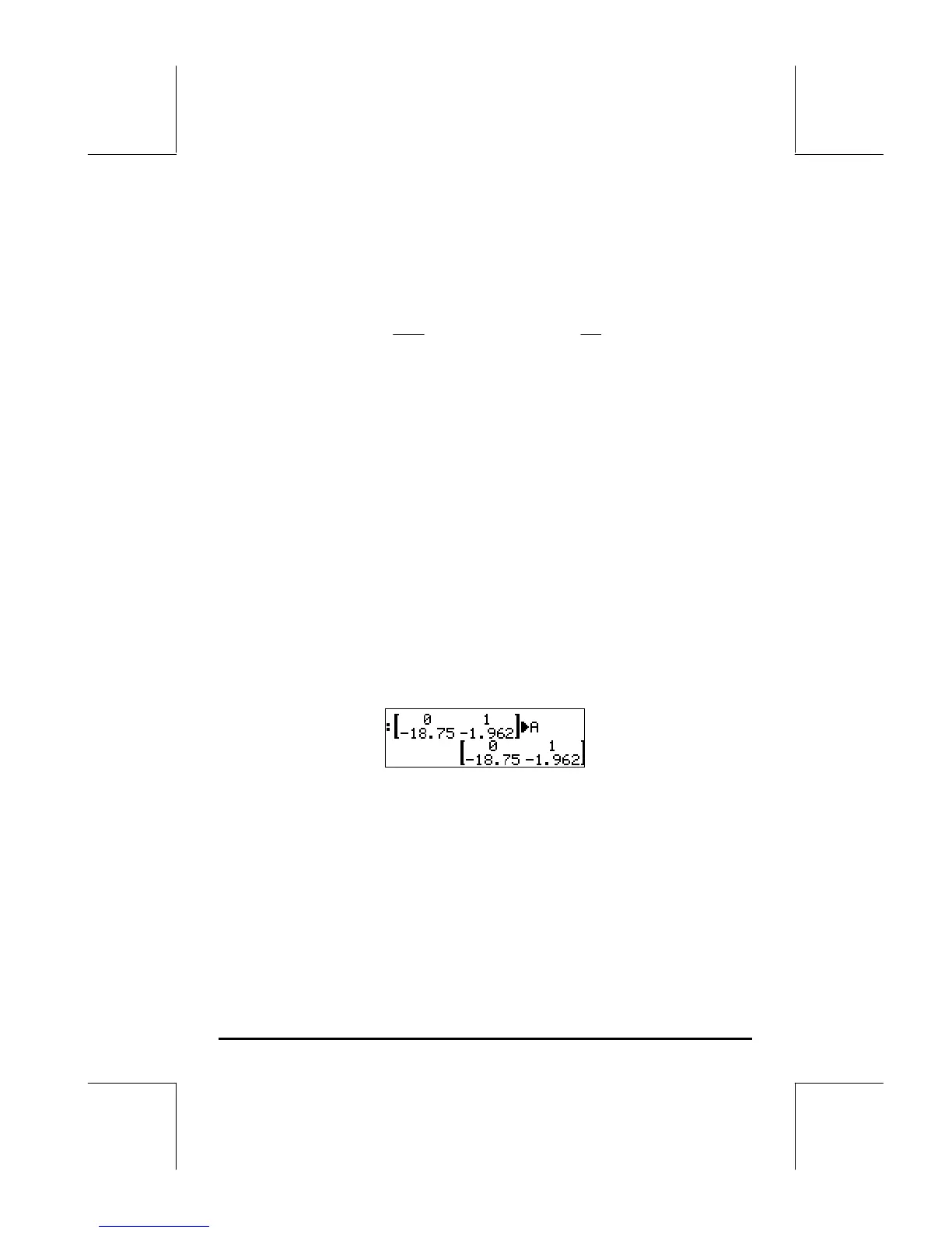
Re-write the ODE as: w' = Aw, where w = [ x x' ]
T
, and A is the 2 x 2
matrix shown below.
⋅
−−
=
'962.175.18
10
'
'
x
x
x
x
The initial conditions are now written as w = [0 6]
T
, for t = 0. (Note: The
symbol [ ]
T
means the transpose of the vector or matrix).
To solve this problem, first, create and store the matrix A, e.g., in ALG mode:
Then, activate the numerical differential equation solver by using: ‚ Ï
˜ @@@OK@@@ . To solve the differential equation with starting time t = 0 and
final time t = 2, the input form for the differential equation solver should look
as follows (notice that the Init: value for the Soln: is a vector [0, 6]):
 Loading...