Synthesis Engine
Synthesis Engine
96 97
State Variable Filter
The second applyable filter to the branches is called the „State Variable Filter“, a tool for
multifunctional subtractive filtering that is fed by an adjustable crossfade mix of both
branch signals. The Comb Filter can be faded into the input mix as well.
The State Variable Filter consists of two two-pole filters with blendable characteristics
(lowpass, bandpass, highpass) which can operate in parallel or in series by a continuously
adjustable amount. In serial mode, the damping slope can be raised from 12 to 24 dB per
octave (becoming a four-pole filter eectively). In parallel applications, the filters can also
be used to create two formants (useful for vowel-like sounds).
The filter frequencies are determined by a tunable center frequency which can be sensi-
tive to Key Tracking and the influence of Envelope C. A Spread parameter determines how
much the individual filter frequencies are shied apart from the center frequency. With no
spreading, one peak emerges at the center frequency. The strength of the peak depends
on the filter resonance, which also can be sensitive to Key Tracking and the influence of
Envelope C. When spreading is applied, the peak splits into two peaks, weakening strong
resonances and creating formants.
The filter type can be continuously blended between an overall lowpass, bandpass and
highpass behavior. In serial mode with a negative spreading, a band-rejecting (notch)
behavior can be achieved as well.
A crossfade mix of both branches can also be applied for frequency modulation.
Parallel behavior can be produced in two ways, by either adding or subtracting the
second filter to/from the first. Subtraction will lead to phase cancellations.
In conclusion, the State Variable Filter is a versatile subtractive filter capable of creating
formants and dierent characteristics.
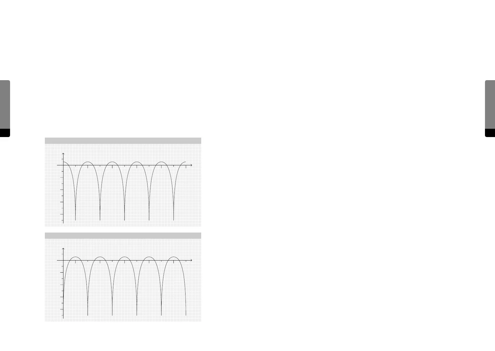
The following diagram shows a simplified frequency response for the Comb Filter.
Consider a tonal signal (with a clear fundamental frequency) which feeds the Comb Filter.
The Comb Filter output is added to the signal (upper graph) or subtracted from the signal
(lower graph).
Both graphs show the typical, generalized frequency response of a comb eect, as shown
by the periodical peaks. The width of the peaks depends on the Comb Filter’s pitch
parameter (equivalent to a delay time), meaning that certain signal frequency compo-
nents will be attenuated and other components will be amplified, depending on the delay
time.
In addition, when subtracting the Comb Filter signal from the incoming signal, the peaks
are shied, and the emerging comb tone will be lowered by one octave.
Comb Filter – Frequency Response
7
Magnitude
(dB)
Frequency
Ratio
Non-inverted Mix
0 dB
– 20 dB
1.0 2.0 3.0 4.0 5.0
0.5 1.5 2.5 3.5 4.5
– 40 dB
– 60 dB
– 80 dB
0 dB
– 20 dB
– 40 dB
– 60 dB
– 80 dB
Magnitude
(dB)
Frequency
Ratio
Inverted Mix