BAS 100B/W - Page 136

10-68
10 SEC
0.1 to 1.0 Hz
10 mV AMP
200 mV FS
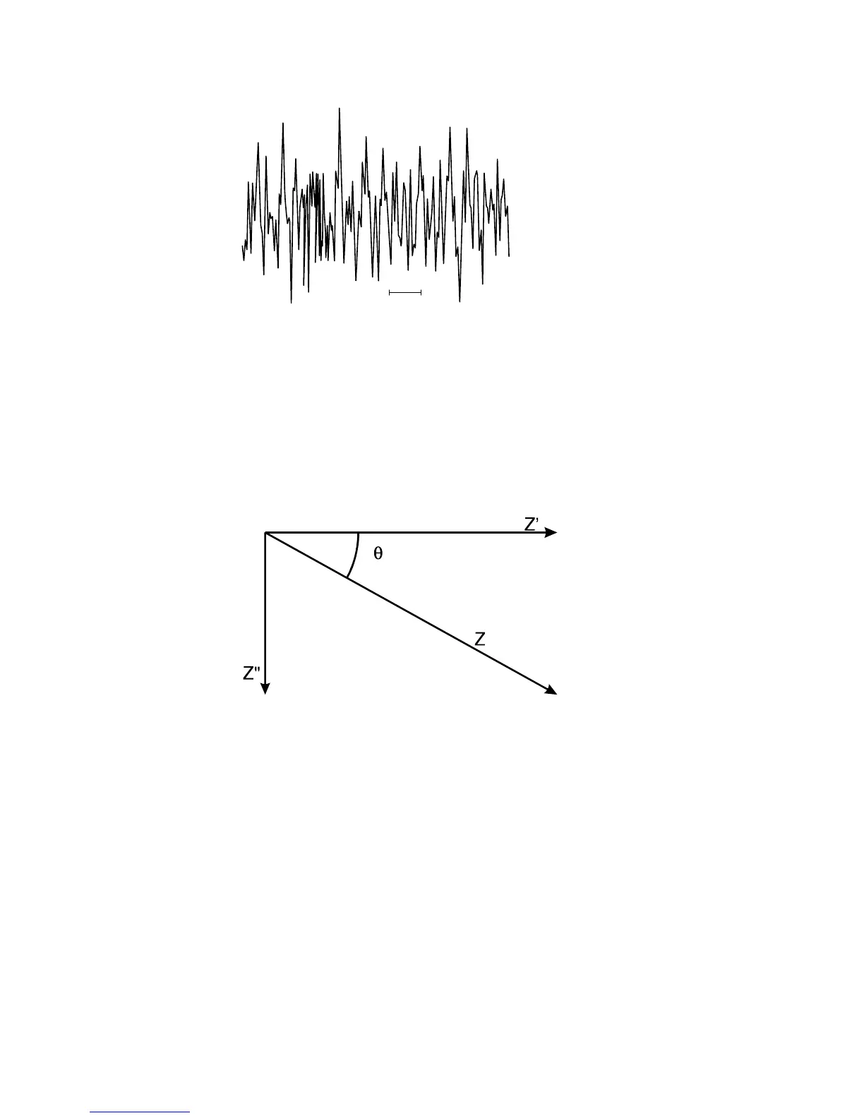
Figure 10-43.
An example of the white noise wave form used for
IMP
.
The presentation of the experimental data is complicated by the phase difference
between the applied potential and the current response. The results can be represented
in terms of impedances (Z where Z = E/I) or admittances (Y where Y = 1/Z). A
vector diagram illustrating the relationship between Z (total impedance), Z' (the
impedance in-phase with the applied potential), Z" (the impedance 90
o
out of phase
the applied potential) and
θ
(the phase angle) is shown in Figure 10-44. It should also
be noted that these parameters vary with frequency (
ω
).
Figure 10-44.
Vector diagram for impedances.
There are 14 impedance plots available on the BAS 100B/W. These are as follows:
1. -Z" - Z' (Nyquist plot)
2. -Y" - Y'
3. Log Z - Log(
ω
) (Bode plot)
4. Log Y - Log(
ω
)
5.
θ
- Log(
ω
) (Bode plot)
6. -Z" & Z' - Log(
ω
)
7. -
ω
Z" -
ω
Z'
8. -
ω
Y" -
ω
Y'
9. -Z"/
ω
- Z'/
ω
10. -Y"/
ω
- Y'/
ω
11. Z' -
ω
Z"