Casio FX-CG10 - Page 75

2-29
k Second Derivative Calculations [OPTN] - [CALC] - [ d
2
/ dx
2
]
After displaying the function analysis menu, you can input second derivatives using the
following syntax.
<Math input/output mode>
K4(CALC)3(d
2
/dx
2
) f(x)ea
or
4(MATH)5(d
2
/dx
2
) f(x)ea
<Linear input/output mode>
K4(CALC) 3( d
2
/ dx
2
) f ( x ) ,a )
a is the point for which you want to determine the second derivative.
Second derivative calculations produce an approximate derivative value using the following
second derivative formula, which is based on Newton’s polynomial interpretation.
In this expression, values for “sufficiently small increments of
h ” are used to obtain a value that
approximates f " ( a ).
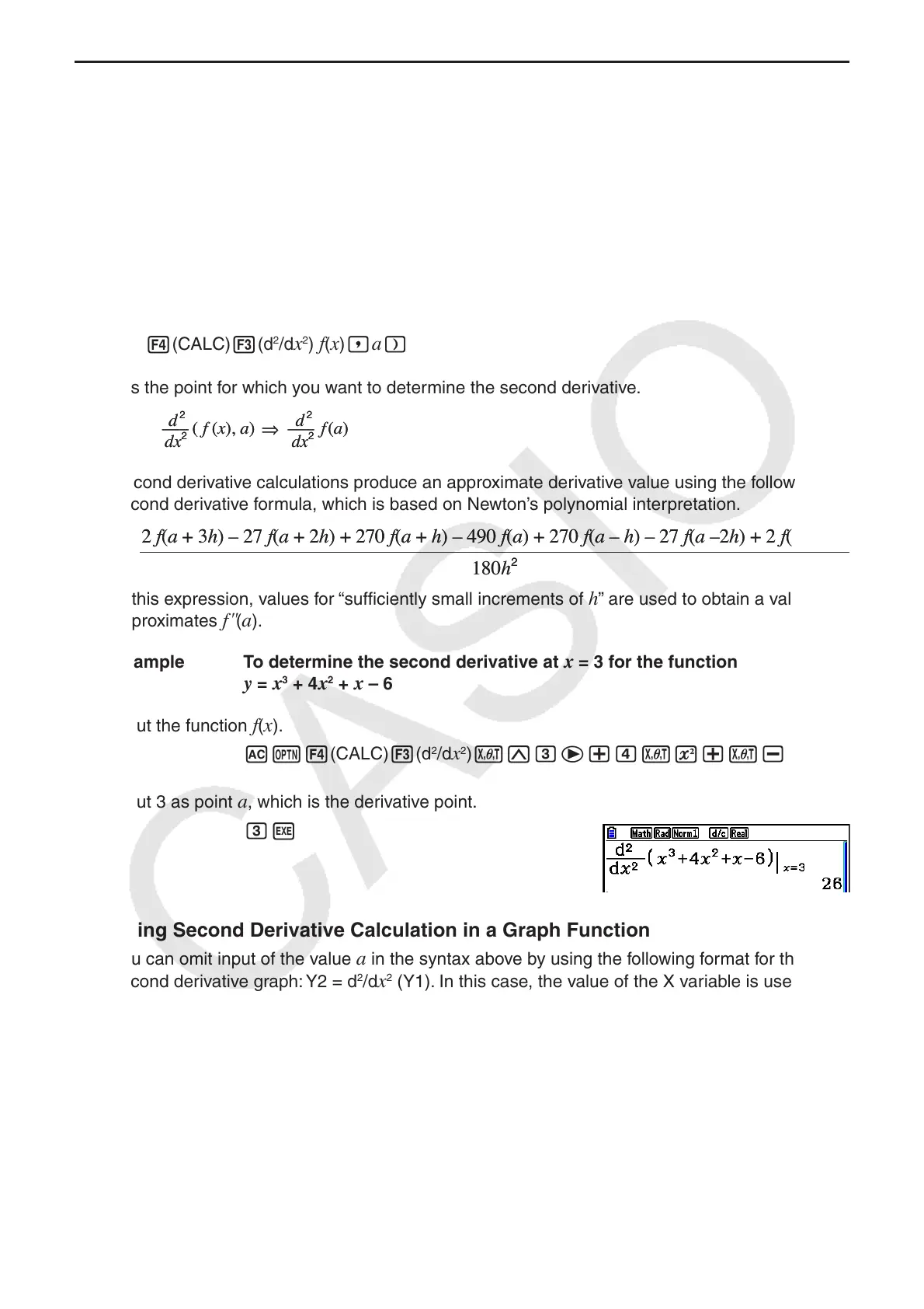
Example To determine the second derivative at
x = 3 for the function
y = x
3
+ 4 x
2
+ x – 6
Input the function f ( x ).
AK4(CALC) 3( d
2
/ dx
2
) vMde+evx+v-ge
Input 3 as point a , which is the derivative point.
dw
Using Second Derivative Calculation in a Graph Function
You can omit input of the value a in the syntax above by using the following format for the
second derivative graph: Y2 = d
2
/dx
2
(Y1). In this case, the value of the X variable is used
instead of the value
a.
Second Derivative Calculation Precautions
The precautions that apply for first derivative also apply when using a second derivative
calculation (see page 2-28).
d
2
d
2
––– (
f
(
x
),
a
)
⇒
–––
f
(
a
)
dx
2
dx
2
d
2
d
2
––– (
f
(
x
),
a
)
⇒
–––
f
(
a
)
dx
2
dx
2
f
''(a) =
180h
2
2 f(a + 3h) – 27 f(a + 2h) + 270 f(a + h) – 490 f(a) + 270 f(a – h) – 27 f(a –2h) + 2 f(a – 3h)
f
''(a) =
180h
2
2 f(a + 3h) – 27 f(a + 2h) + 270 f(a + h) – 490 f(a) + 270 f(a – h) – 27 f(a –2h) + 2 f(a – 3h)