–
Press Pacing time and enter a new value
if you want to change the default value
20 ms. The range is 2 ms - 1000 s. The
pacing parameter sets the sampling inter
-
val.
–
Activate the set pacing time by pressing
Pacing Off. The status is changed to
Pacing On. Status Pacing Off means that
the set number of samples will be taken
with minimum delay.
–
Press HOLD/RUN to stop the measuring
process.
–
Press RESTART to initiate one data cap
-
ture
–
Toggle STAT/PLOT to view the measure
-
ment result as it is displayed in the differ-
ent presentation modes.
+
Note that you can watch the in-
termediate results update the
display continually until the com-
plete data capture is ready.
This is particularly valuable if the
collection of data is lengthy.
Measuring Speed
When using statistics, you must take care that
the measurements do not take too long time to
perform. Statistics based on 1000 samples
does not give a complete measurement result
until all 1000 measurements have been made,
although it is true that intermediate results are
displayed in the course of the data capture.
Thus it can take quite some time if the setting
of the counter is not optimal.
Here are a few tips to speed up the process:
–
Do not use AUTO trigger. It is convenient,
but it takes a fraction of a second each
time the timer/counter determines new
trigger levels, and 1000 or 10000 times a
fraction of a second is a long time.
–
Do not use a longer measuring time than
necessary for the required resolution.
–
Remember to use a short pacing time, if
your application does not require data col
-
lection over a long period of time.
Determining Long or Short
Time Instability
When making statistical measurements, you
must select measuring time in accordance
with what you want to obtain:
Jitter or very short time (cycle to cycle) varia
-
tions require that the samples be taken as Sin
-
gle measurements.
If average is used (Freq or Period Average
only), the samples used for the statistical cal-
culations are already averaged, unless the set
measuring time is less than the period time of
the input signal (up to 160 MHz). Above this
frequency prescaling by two is introduced
anyhow, and as a consequence a certain
amount of averaging. This can be a great ad-
vantage when you measure medium or long
time instabilities. Here averaging works as a
smoothing function, eliminating the effect of
jitter.
The signal in Fig. 6-1contains a slower varia
-
tion as well as jitter. When measuring jitter
Process
6-4 Statistics
T i m e
T i m e I n t e r v a l
o r F r e q u e n c y
J i t t e r
D r i f t
Fig. 6-1 Jitter and drift.
 Loading...