PVB = 500,5000,500
1
st
point in Figure 6.21 - B axis
PVA = 1000,4000,1200
2
nd
point in Figure 6.21 - A axis
PVB = 4500,0,1200
2
nd
point in Figure 6.21 - B axis
PVA = 1000,4000,750
3
rd
point in Figure 6.21 - A axis
PVB = -1000,1000,750
3
rd
point in Figure 6.21 - B axis
BTAB
Begin PVT mode for A and B axes
PVA = 800,10000,250
4
th
point in Figure 6.21 - A axis
PVB = 200,1000,250
4
th
point in Figure 6.21 - B axis
PVA = 4000,0,1000
5
th
point in Figure 6.21 - A axis
PVB = -900,0,1000
5
th
point in Figure 6.21 - B axis
PVA = 0,0,0
Termination of PVT buffer for A axis
PVB = 0,0,0
Termination of PVT buffer for B axis
EN
NOTE: The BT command is issued prior to filling the PVT buffers and additional PV commands are added during motion for demonstration purposes
only. The BT command could have been issued at the end of all the PVT points in this example.
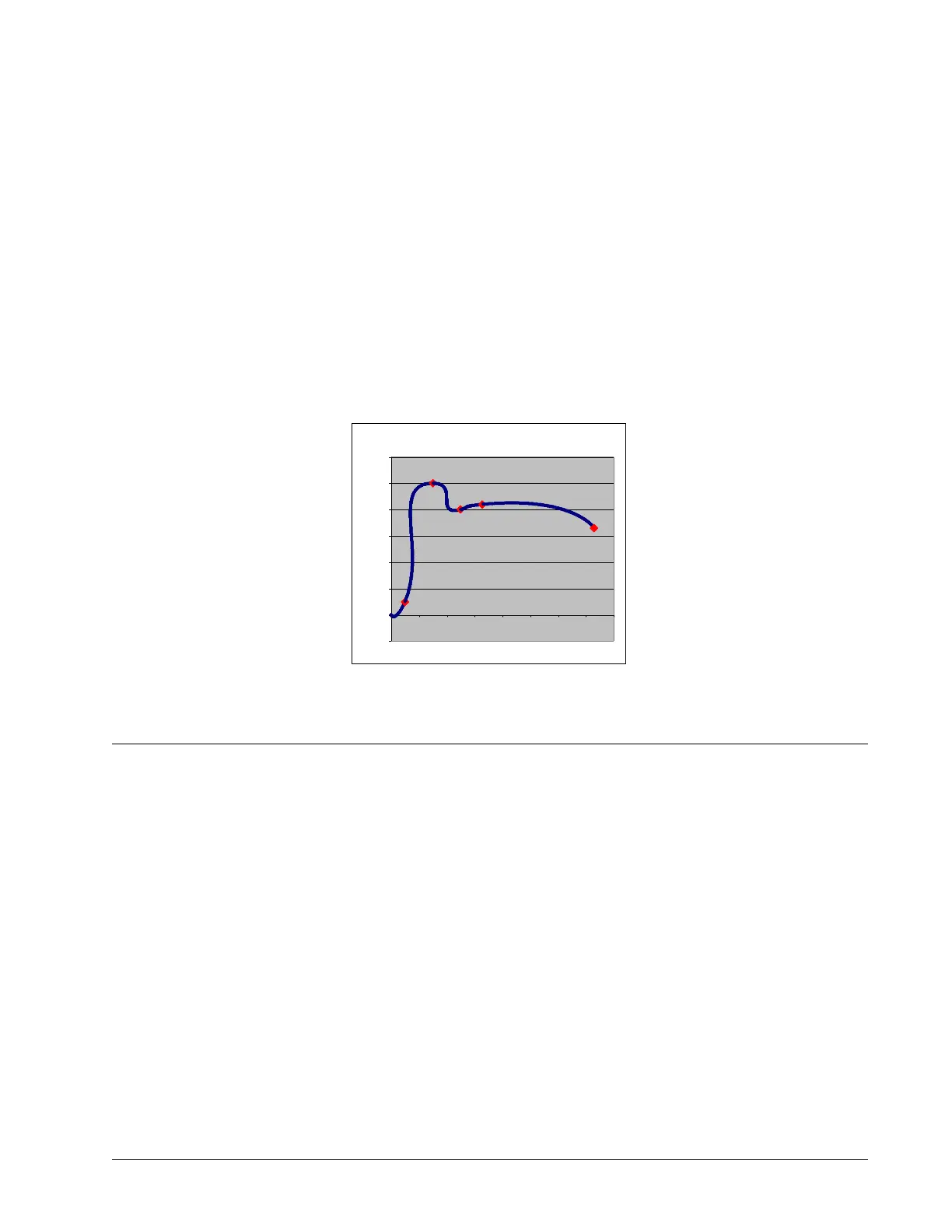
The resultant X vs. Y position graph is shown in Figure 6.17, with the specified PVT points enlarged.
Contour Mode
The DMC-41x3 also provides a contouring mode. This mode allows any arbitrary position curve to be prescribed
for 1 to 8 axes. This is ideal for following computer generated paths such as parabolic, spherical or user-defined
profiles. The path is not limited to straight line and arc segments and the path length may be infinite.
Specifying Contour Segments
The Contour Mode is specified with the command, CM. For example, CMXZ specifies contouring on the X and Z
axes. Any axes that are not being used in the contouring mode may be operated in other modes.
A contour is described by position increments which are described with the command, CD x,y,z,w over a time
interval, DT n. The parameter, n, specifies the time interval. The time interval is defined as 2
n
sample period (1 ms
for TM1000), where n is a number between 1 and 8. The controller performs linear interpolation between the
specified increments, where one point is generated for each sample. If the time interval changes for each
segment, use CD x,y,z,w=n where n is the new DT value.
Consider, for example, the trajectory shown in Figure 6.18. The position X may be described by the points:
Point 1 X=0 at T=0ms
Point 2 X=48 at T=4ms
Chapter 6 Programming Motion ▫ 85 DMC-41x3 User Manual
Figure 6.17: X vs Y Commanded Positions for Multi-Axis
Coordinated Move
X vs Y Commanded Positions
-1000
0
1000
2000
3000
4000
5000
6000
0 1000 2000 3000 4000 5000 6000 7000 8000