Measurement
HINT
To get a better understanding of the aliasing effect, we recommend to take the DEWESoft®
PRO training course: Spectral analysis using the FFT:
http://www.dewesoft.com/pro/course/spectral-analysis-using-the-fft-29
Our professional online training courses are available free of charge to registered users of our
homepage.
Anti-aliasing
To avoid aliasing, we must cut all frequencies that are higher than half of the sample rate. But on the other hand, we do
not want to damp the amplitude of the signal below the Nyquist frequency. To meet both goals, we need a filter (in this
context called: anti-aliasing filter) with sharp damping at half of the sampling rate (which requires a high order filter).
6.1.1.5 Aliasing-free Bandwidth
In the previous chapters we have learned, that an ideal filter with infinitely sharp filter characteristics is not possible in
real-world applications.
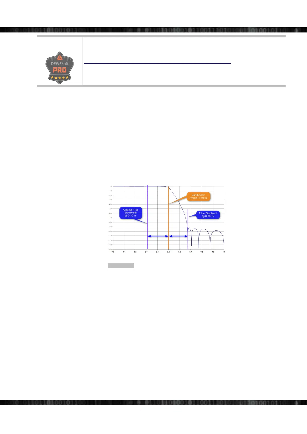
The frequency response in Illustration 181 below shows the bandwidth (-3dB point) at about half of the sampling rate
(Nyquist criteria). All frequencies higher than the Nyquist frequency will be folded back. But the frequencies above the
Filter Stopband are already attenuated so much, that they are negligible. Thus, the only guarantee that can be made, is
that all frequencies in the aliasing free bandwidth are correct.
Amplitude [dB]
Frequency (normalised to Fs)
Illustration 181: Bandwidth vs. Aliasing-free Bandwidth
Illustration 181 above shows the filter characteristics relative to the sample rate. To make it easier to understand, let's
make an example with some concrete values. Let's assume a sampling rate of 1kS/sec. The bandwidth of this low-pass
filter is at 500kHz. All input frequencies between 500Hz and 680Hz (=0.68*1kHz) can be folded back to the 320Hz to
500Hz range. All input frequencies higher than 680Hz are rejected by the filter anyway and can be ignored. Thus, the
aliasing free bandwidth is 320Hz (since the range of 320Hz and 500 can already be due to the aliasing effect).
6.1.1.6 Filter technologies
Different technologies can be used to realise a filter. In this context we only need to consider two technologies:
analogue and digital filters.
Analogue filters
Analogue filters are composed of passive electronics (i.e. capacitors, inductors, resistors) and operator on continuously
varying signals. They can be described with linear differential equations: thus they are also called passive linear
analogue electronic filters.
Good analogue filters are inherently difficult to design and even when you select all components carefully, 8th order is
the best you can implement without significant inter-channel phase-mismatch.
Doc-Version: 1.4.2 www.dewesoft.com Page 129/166