Chapter 12: Statistics 179
Since the scatter plot of time-versus-length data appears to be approximately linear, fit a line to the
data.
4. Press 6 Ë 5 Í to store the first pendulum
string length (6.5 cm) in
L1. The rectangular cursor
moves to the next row. Repeat this step to enter
each of the 12 string length values in the table.
5. Press ~ to move the rectangular cursor to the first
row in
L2.
Press Ë 51 Í to store the first time
measurement (.51 sec) in
L2. The rectangular
cursor moves to the next row. Repeat this step to
enter each of the 12 time values in the table.
6. Press o to display the Y= editor.
If necessary, press ‘ to clear the function Y1.
As necessary, press }, Í, and ~ to turn off
Plot1, Plot2, and Plot3 from the top line of the
Y= editor (Chapter 3). As necessary, press †, |,
and Í to deselect functions.
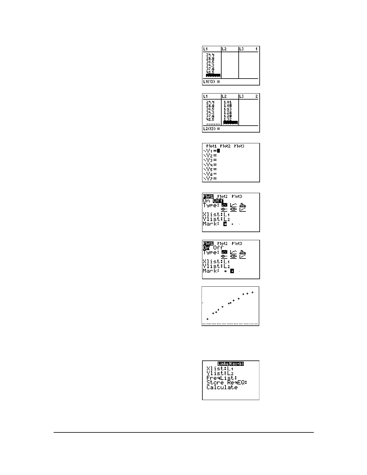
7. Press y , 1 to select 1:Plot1 from the
STAT PLOTS menu. The stat plot editor is
displayed for plot 1.
8. Press Í to select On, which turns on plot 1.
Press
† Í to select " (scatter plot). Press
† y d to specify Xlist:L1 for plot 1. Press
† y e to specify Ylist:L2 for plot 1. Press
† ~ Í to select + as the Mark for each data
point on the scatter plot.
9. Press q 9 to select 9:ZoomStat from the ZOOM
menu. The window variables are adjusted
automatically, and plot 1 is displayed. This is a
scatter plot of the time-versus-length data.
10. Press … ~ 4 to select 4:LinReg(ax+b) (linear
regression model) from the
STAT CALC menu.

 Loading...


