conductivity (the result of the inversion) between depth 1.5 m and 2.0 m.
The apparent conductivity is distributed so that the conductivity of the
shortest dipole is situated into the zero depth, the conductivity of the
biggest dipole is situated into the maximum depth and the conductivity of
the middle dipole is situated into the middle layer. The contouring
software must be set to omit -999 values (e.g. “z=-999”), because
this value is used to differentiation conductivity inversion which was not
possible to calculate successfully (measured conductivities were out of
range for inversion calculation – over 1000 mS/m, under 1 mS/m - or too
wide difference between measured conductivities).
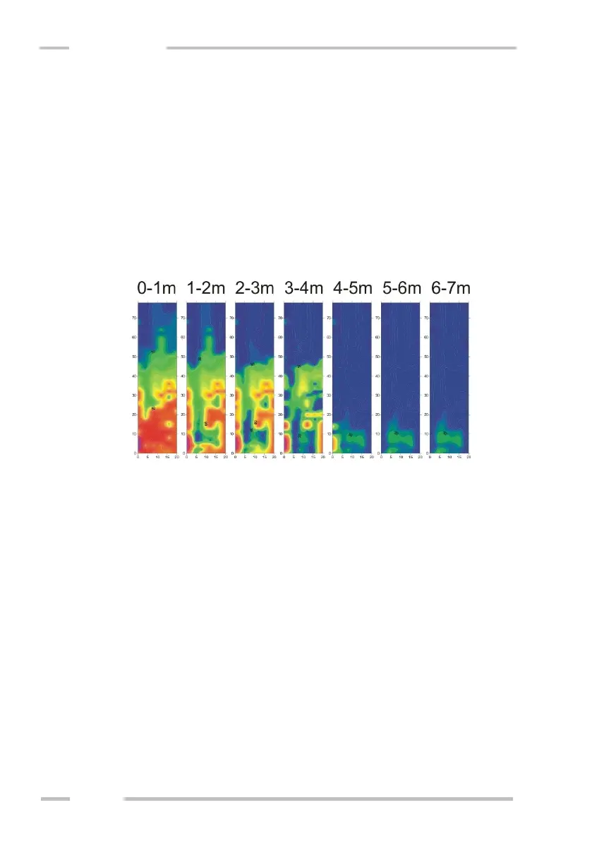
True conductivity depth slices example:
Recommended setting for .srf_map exporting:
CMD-Explorer / High depth range: 6 m / 6 (12) layers
CMD- Explorer / Low depth range: 3 m / 6 layers
CMD-MiniExplorer / High depth range: 2 m / 6 (12) layers
CMD-MiniExplorer / Low depth range: 1 m / 6 layers
- .interpolated.srf_map.dat is ASCII file like “.srf_map.dat”. This file is
generated only from continuous measurements (both manual and GPS).
The positions of measured points without primary position information
(data measured between length marks or between valid GPS data
positions) are interpolated between data with known positions.