RoentDek DLD40 - Page 9

X = x1 – x2 + O
x
and Y = y1 - y2 + O
y
Equation 1.1
with x1, x2, y1 and y2 denominating the time for each signal, O
x
and O
y
are arbitrary offsets.
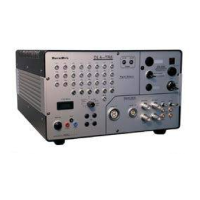
The fast timing signal picked up from an MCP contact or, in the case of a pulsed particle/photon source, a “machine trigger”
signal can serve as time reference. The single pitch propagation time (for 1mm) on the delay line is about 0.75ns for DLD40,
1ns for DLD80 and 1.24ns for DLD120. Thus the correspondence between 1mm position distance and relative time delay in
the 2d image is twice this value: about 1.5ns, 2ns or 2.5ns, respectively. Note that these numbers are only accurate within 5%
and are slightly different for each dimension. In order to calculate the position in mm from the digital X and Y values you have
to take into account the bin width of your TDC and the single pitch propagation time for the respective layer.
Figure 1.1: Operation principle of the delay-line-anode,
left picture from: Sobottka and Williams IEEE TS-35 (1988) 348
The Hexanode has an additional layer and gives over-determined (redundant) position information: It is possible calculating
the two-dimensional particle position of signals from of any two of the tree layers. The signals from the third layer serve as a
redundant source of information for cases when signals are “lost” due to electronic dead-time (multiple hit events), non-
continuous winding schemes (anode with central holes) or non-perfect electronic threshold conditions/damping on special
very large delay-line anodes. With the Hexanode it is also possible to control their delay-lines’ intrinsic resolution and linearity,
improving the overall imaging performance. The Hexanode’s coordinate frame u, v, w can be transformed into a Cartesian
coordinate system by the following equations using only two of the hexagonal coordinates respectively, if the connection
scheme in the next section is chosen:
X
uv
=
Oxu +
Y
uv
=
( )
y O
vu +
− 2
3
1
X
uw
= X
uv
Y
uw
=
( )
y Ouw +−2
3
1
X
vw
=
( )
x O++ wv
Y
vw
=
( )
yOv
w +−
3
1
Equation 1.2
O
x
and O
y
are arbitrary offsets. The position in a hexagonal coordinate frame is coded by the arriving time differences from
signals in opposite corners of the anode as in case of the DLD.
u = (x1 – x2) * d1
v = (y1 – y2) * d2
w = (z1 – z2) * d3 + o
Equation 1.3
If 1/v
i
is the single pitch propagation time for a delay line layer i (v
i
is slightly different for each layer) then d
i
is given by
MCP Delay Line Detector Manual (11.0.1304.1) Page 9 of 83