NIRStar 14.1 - User Manual
Page 103 of 124
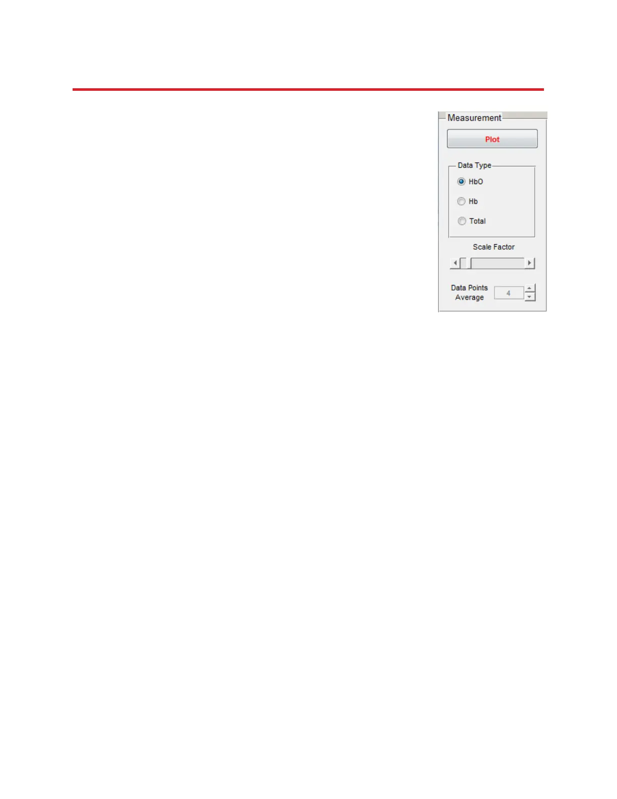
Data Type:
Select the Hb-state to be shown in the MATLAB display (HbO: Oxy-Hemoglobin;
Hb: Deoxy-Hemoglobin; Total: Total Hemoglobin, i.e. the sum of Hb and HbO).
Scale Factor:
This slider may be used to adjust the amplitude scale of the topographic plot.
Data Points Average:
The time average (specified in data points) determines the number of scans
that the software averages between successive display updates. The display
rate for the advanced display will be reduced accordingly. You may use this
feature to slow down the display rate to conserve computational power, or as
means of reducing high-frequency signal components (heartbeat, noise).
18.2.2 Quick Guide
Setting up a 2D/3D/Cortex-Plot
1. Make sure the standalone topographic rendering functionality is installed; run NIRStar
2. Call Hardware Configuration → Displays Setup; click on ‘Launch GUI’; close Hardware
Configuration.
3. In the ‘GUI’ dialog select Run Probe Setup → either define a new ProbeInfo file (and
proceed to step 4), or load an existing ProbeInfo file (go to step 5).
4. After the channel positions have been defined, click on ‘Save & Close’ at the bottom of
the ‘Probe Setup’ GUI and enter an appropriate file name (*_probeInfo.mat).
5. Close the ‘Probe Setup’ GUI and choose the desired plotting mode (2D, 3D or Cortex) in
the Plot Mode module of the ‘GUI’ interface.
6. Click on the Prepare Display button. The ‘Prepared?’ indicator should change from red to
green, and a plot window should open.
7. Keeping the plot window open, proceed with standard NIRStar gain setup to prepare for
the measurement.
8. Start the scan (Preview or Record). The recorded data will be automatically displayed.
9. In the ‘GUI’ interface, click on ‘Plot’ to start the rendering display. You may adjust the
display properties (type, scaling, averaging) as desired.
10. The plot display will stop at the end of the measurement.